Z-Transform |
|---|
DefinitionThe Z-transform is just a discrete-time equivalent of the Laplace transform i.e. a power series representation of a discrete-time interval data. If the function $x(n)$ is defined for discrete values of $n$ (n=0,1,2,3,..) and $x(n)=0$ for $k<0$, then Z-transform for the same is given by: \[Z\{ x(n)\} =\sum _{ n=0 }^{ \infty }{ x(n){ z }^{ -n } }\] where $z=r{ e }^{ s j }$ Here $z$ is simply some complex number with $s$ as a complex argument ($s=\sigma +j\omega $),$r$ as its magnitude and The above transform is also referred to as Unilateral Z-transform as we are considering only a single side (The non-negative side) of $n$. The two-sided Z-transform (n=...,-2,-1,0,1,2...) is given by: \[Z\{ x(n)\} =\sum _{ n=-\infty }^{ \infty }{ x(n){ z }^{ -n } }\] We usually represent the obtained Z-transform of $x(n)$ as $X(n)$. 1 |
MotivationTill now we have come across various transforms such as Laplace Transform, Continuous Fourier Transform, Discrete Fourier Transform. In Continuous Fourier Transform, we saw how we can get a frequency domain function from a continuous-time domain function using only the sinusoids(${ e }^{ j\omega }$). Now since the time could be sometimes considered in discrete intervals, we have Discrete Fourier Transform for the same objective. In Laplace Transform, we simply even consider exponentials along with sinusoids (i.e. ${ e }^{ \sigma +j\omega }$) to convert into a frequency domain function. Now is there any way to represent a function(in discrete time intervals) in terms of sinusoids as well as exponentials? Now we might ask for our need to represent a function in discrete time intervals. And how can time be considered as discrete? Consider copying some data (say some music) into a CD. How can we copy or rather store the data (amplitude, frequency, and pitch of tones in this case) defined in continuous time (i.e. infinite data points!)? We try to find what exactly the term discrete time intervals mean and how Z-transforms are carried out over them. 2 |
|
3 |
|
Video 1 : Sampling of a Continuous time function |
Bird's eye viewSince we already have Laplace transform to represent a continuous function in terms of sinusoids as well as exponentials, we simply modify Laplace transform to calculate in discrete time intervals. Therefore Z-transform can be thought of as a modification to Laplace transform. Alternatively, Z-transform can be thought of as a generalization of Discrete Fourier Transform by introducing a real number $A$. As Laplace transforms themselves are a generalization for Continuous Fourier Transform by introducing exponential (${ e }^{ \sigma }$) which is some real number, therefore generalizing the Discrete Fourier Transform would serve our purpose. Although many physical systems have data inherently in discrete-time(for example lowest temperatures of a set of days), in many of the cases, data indeed is defined in continuous time. Hence it is made into discrete through a process called sampling (refer context for detailed view). Above all, Z-transforms also makes it easier in terms of notation as compared to Laplace Transforms. 4 |
Context to the DefinitionSampling is a method used to represent continuous-time data in discrete forms. The following image is a simple intuition of an analog to digital converter, a device used for the above purpose. Here $f(t)$ is a continuous function and ${ f }^{ * }(t)$ is its discrete form. 5 |
|
6 |
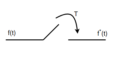
Image 1 : Sampling of a function with intervals of T [Created using 'App.Diagrams'] |
|
Since the frequency of samples taken is usually very high, therefore it is assumed that the obtained function takes in any value. (which makes it partially continuous!) As Z transform is a generalization of Discrete Fourier Transform by simply taking the amplitude as $1$, Thus we can say that the Discrete-Time Fourier transform is a Z transform when computed on the unit circle. Since the obtained transform is a complex function, therefore to represent it graphically, we need four planes. Two-planes to represent the input (real and imaginary parts) and similarly two for the output. Therefore to avoid imagining the complex 4-D plane, we consider the input on one pair of axes and output on another pair. Consider the Z-transform of $f(t) = 2{ \delta }_{ 0 }(t)+3{ \delta }_{ 1 }(t)+4{ \delta }_{ 2 }(t)$ 7 |
|
10 |
|
Video 2 : Z Transform of a delta function |
|
Since the obtained transform satisfies for any magnitude of $z$ (i.e. for any $z$ ), except for $z=0$, we say the transform Converges! Here the data set ($x[n]$) could even be an infinite set. If it is a finite set, then the transform becomes easier as it would be just multiplication of each point with a complex number. But when it is an infinite set, we start to deal with infinite summations! Since whenever we deal with infinite summations with a variable ($z$ in this case), there might exist only certain ranges of $z$ for which the sum converges. This range of values of $z$ for which the summation converges is referred to as Region Of Convergence. i.e. \[ROC=\left\{ z:\left| \sum _{ n=-\infty }^{ \infty }{ x[n]{ z }^{ -n } } \right| <\infty \right\}\] Consider the data set, $x[n]=(0.5)^{ n }$ for $n=0,1,2..$ . Let us analyze its Region Of Convergence! 11 |
|
14 |
|
Video 3 : Region Of Convergence for the given transform |
Applications
15 |
HistoryThe idea of Z-transform dates back to 1730 when De Moivre used the concept of “Generating Functions” to encode a given function. He multiplied each point of the data set with a specific function to change its form. Though there wasn’t any formalized form for the same. In 1947, W. Hurewicz used a special kind of transform for solving linear constant-coefficient difference equations. (by transforming the sampled sequence). Similarly, in 1952, Lotfi Zadeh and Ragazzini who are also the members of the sampled-data control group at Columbia University used a similar transform. They formalized the results and termed it as Z-Transform. Since it wasn’t taking care of the ideal delays that aren’t multiples of the sampling time, E.I Jury later modified and formulated its modified version as advanced Z-transform. 16 |
References
16 |
Further Readings
16 |
| Contributor: |
| Mentor & Editor: |
| Verified by: |
| Approved On: |
The following notes and their corrosponding animations were created by the above-mentioned contributor and are freely avilable under CC (by SA) licence. The source code for the said animations is avilable on GitHub and is licenced under the MIT licence.
