The TNB Frame and Serret–Frenet Formulae |
|---|
DefinitionFor any $t = t_0$, three mutually orthogonal unit vectors, $\overrightarrow{T}(t_0), \overrightarrow{N}(t_0), \overrightarrow{B}(t_0)$ define an orthonormal basis for the 3-dimensional coordinate system: for any vector $\overrightarrow{v}$ we can write it as: $$\overrightarrow{v} = (\overrightarrow{v}\cdot\overrightarrow{T}(t_0))\overrightarrow{T}(t_0) + (\overrightarrow{v}\cdot\overrightarrow{N}(t_0))\overrightarrow{N}(t_0) + (\overrightarrow{v}\cdot\overrightarrow{B}(t_0))\overrightarrow{B}(t_0)$$ This basis is called the TNB frame or Frenet-Serret frame of the curve at $t = t_0$.
MotivationIn a plane curve, the curvature suffices to describe how a curve changes along its length. In three dimensions, only the curvature is not sufficient to describe how a curve is changing along its length, and another coefficient called torsion is required to give an understanding of how the curve "twists" in a particular direction. In the Frenet frame moving smoothly along a curve, the derivative of the $\overrightarrow{N}$ gives a particular combination of $\overrightarrow{B}$ and $\overrightarrow{T}$, which will be discussed below. The combination involves the curvature and the torsion. The torsion signifies how much the Frenet frame is twisting around $\overrightarrow{T}$, i.e., how much $\overrightarrow{B}$ and $\overrightarrow{N}$ rotate into each other. The curvature signifies how much $\overrightarrow{T}$ is rotating back into $\overrightarrow{N}$. A relatable example would be of a spiral parking lot. A vehicle going upward in the parking lot would have its normal vector pointing towards the centre of the spiral (the centripetal force), while the tangent vector would denote the velocity of the vehicle, and the binormal vector would denote the upward force exerted by the surface of the spiral, on which the vehicle is moving. Bird's Eye ViewWhat do the tangent line and velocity have in common? Notice how they are both parallel to $r\prime (t)$ and $T(t)$; and are also both orthogonal to $N(t)$ and $B(t)$. Through the course of these notes, we explore whether this implication is actually an inference. A well-known intuitive reference frame, called the Frenet frame, consists of a unit length tangent, $\overrightarrow{T}$, to the central axis, a principal normal, $\overrightarrow{N}$, and a binormal, $\overrightarrow{B}$. Since we know that the tangent and normal vectors to a curve at a given point are unique, the TNB frame thus formed at a point is unique. Visually, these three vectors along with the plane prescribed by the former two can be represented as: 1 |
|
2 |
|
Figure 1: Creation of a TNB frame |
Context of the DefinitionWe know that for the vector function $\overrightarrow{r}(t)$, the tangent vector (provided it exists) is given by $\overrightarrow{r}\prime (t)$. The unit tangent vector to the curve is given by: $$T(t) = \frac{\overrightarrow{r}\prime (t)}{\left|\left|\overrightarrow{r}\prime (t)\right|\right|}$$ The tangent vector gives an indication of how a moving point would travel along the given curve. The unit vector orthogonal to the tangent vector is called the unit normal vector and is given by: $$\overrightarrow{N}(t) = \frac{\overrightarrow{T}\prime (t)}{\left|\left|\overrightarrow{T}\prime (t)\right|\right|}$$ It is important to understand that the normal vector and tangent vector prescribe a plane (shown in Figure 1), which twists as a point moves along the curve. The vector which is normal / perpendicular to this plane is called the binormal vector, and is given by: $$\overrightarrow{B}(t) = \overrightarrow{T}(t) \times \overrightarrow{N}(t)$$ The animations below depict: the plane prescribed by the unit normal and unit tangent vectors; and the TNB frame of a curve at each point respectively. 3 |
|
4 |
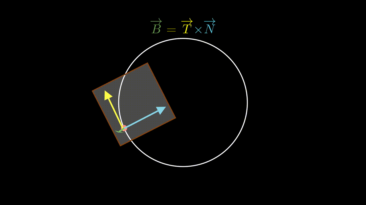
Figure 2: Visualization of $\overrightarrow{T}$, $\overrightarrow{N}$ and $\overrightarrow{B}$ |
|
5 |
|
Figure 3: TNB frame for points along a helix |
The Serret-Frenet FormulaeLet us discuss these formulae while solving an example along with the explanation. Consider the curve $r(t) = \left\langle a\cos{t}, a\sin{t}, bt\right\rangle$. A few inferences from the curve's equation: $$r\prime (t) = \left\langle -a\sin{t}, a\cos{t}, b\right\rangle$$ $$T(t) = \frac{r\prime (t)}{\left|r\prime (t)\right|} = \left\langle\frac{-a\sin{t}}{\sqrt{b^{2} + a^{2}}}, \frac{a\cos{t}}{\sqrt{b^{2} + a^{2}}}, \frac{b}{\sqrt{b^{2} + a^{2}}}\right\rangle$$ $$T\prime(t) = \left\langle\frac{-a\cos{t}}{\sqrt{b^{2} + a^{2}}}, \frac{-a\sin{t}}{\sqrt{b^{2} + a^{2}}}, 0\right\rangle$$ $$N = \frac{T\prime (t)}{\left|T\prime (t)\right|} = \left\langle -\cos{t}, -\sin{t}, 0\right\rangle$$ $$B = T\times N = \left\langle\frac{b\sin{t}}{\sqrt{a^{2} + b^{2}}}, \frac{-b\cos{t}}{\sqrt{a^{2} + b^{2}}}, \frac{a}{\sqrt{a^{2} + b^{2}}}\right\rangle$$ $$B\prime = \left\langle \frac{b\cos{t}}{\sqrt{a^{2} + b^{2}}}, \frac{b\sin{t}}{\sqrt{a^{2} + b^{2}}}, 0\right\rangle = -\tau N$$ where $\tau$ is some coefficient (discussed below). We know that the curvature, $\kappa = \left|\frac{d\overrightarrow{T}}{ds}\right|$. Assuming that $\kappa\neq 0$, the unit normal vector is defined as $\overrightarrow{N} = \kappa\frac{d\overrightarrow{T}}{ds}$, i.e.: $$\begin{equation}\frac{d\overrightarrow{T}}{ds} = \kappa\overrightarrow{N}\tag{1}\end{equation}$$ Hence, equation (1) means that the tangent vector "curves" into the normal vector. This is depicted in the animation below. 6 |
|
7 |
|
Figure 4: Significance of $\frac{d\overrightarrow{T}}{ds} = \kappa\overrightarrow{N}$ |
|
Intuitively, we can comprehend why the normal vector's direction is inwards at an arbitrary point on a given curve, and that it points to the centre of curvature for that point. Notice how the $z$-component of $\overrightarrow{N}$ is 0 $\implies$ it points to the axis of the cylinder horizontally. Computing $\frac{d\overrightarrow{B}}{ds}$, we get: $$\frac{d\overrightarrow{B}}{ds} = \frac{d(\overrightarrow{T}\times\overrightarrow{N})}{ds} = \overrightarrow{N}\times\frac{d\overrightarrow{T}}{ds} + \overrightarrow{T}\times\frac{d\overrightarrow{N}}{ds}$$ We know, $\frac{d\overrightarrow{T}}{ds} = \kappa\overrightarrow{N}$. Hence, $$\frac{d\overrightarrow{B}}{ds} = \overrightarrow{T}\times\frac{d\overrightarrow{N}}{ds}$$as $\kappa\overrightarrow{N}\times\overrightarrow{N} = 0$ This means, $\frac{d\overrightarrow{B}}{ds}$ is orthogonal to $\overrightarrow{T}$ as well as $\overrightarrow{B}$, meaning: $\frac{d\overrightarrow{B}}{ds}$ is parallel to $\overrightarrow{N}$, i.e.:$$\begin{equation}\frac{d\overrightarrow{B}}{ds} = -\tau\overrightarrow{N}\tag{2}\end{equation}$$ This means that the binormal vector "twists" into the normal vector. This is depicted in the animation given below. 8 |
|
9 |
|
Figure 5: Torsion intuition |
|
In the above example (at the beginning of this section), notice how the torsion, as well as curvature, have a constant value. This means that the curve in the example (a helix) twists, and bends (respectively) at a constant rate. $$\tau = -\frac{d\overrightarrow{B}}{ds}\cdot\overrightarrow{N}$$ is called torsion, and is the rate of change of the curve's osculating plane ($\overrightarrow{B}$). In layman's terms, as curvature measures how much a curve bends as it is traced out: similarly, torsion measures the degree of "twisting" of a curve. This is depiccted in the animation given below. 10 |
|
11 |
|
Figure 6: Significance of $\frac{d\overrightarrow{B}}{ds} = -\tau\overrightarrow{N}$ |
|
We know that $\frac{d\overrightarrow{N}}{ds} = \frac{d(\overrightarrow{B}\times\overrightarrow{T})}{ds} = \overrightarrow{B}\times\frac{d\overrightarrow{T}}{ds} + \frac{d\overrightarrow{B}}{ds}\times\overrightarrow{T}$ $$\implies\frac{d\overrightarrow{N}}{ds} = -\tau \overrightarrow{N}\times\overrightarrow{T} + \overrightarrow{B}\times (\kappa\overrightarrow{N}) = \tau\overrightarrow{B} + \kappa\overrightarrow{B}\times\overrightarrow{N}$$ $$\begin{equation}\implies\frac{d\overrightarrow{N}}{ds}= -\kappa\overrightarrow{T} + \tau\overrightarrow{B}\tag{3}\end{equation}$$ 12 |
|
13 |
|
Figure 7: Significance of $\frac{d\overrightarrow{N}}{ds} = -\kappa\overrightarrow{T} + \tau\overrightarrow{B}$ | $\frac{d\overrightarrow{N}}{ds}$ is orthogonal to $\overrightarrow{N}$ and shows how fast $\overrightarrow{N}$ changes with the arc length |
|
The above derived formulae are called the Frenet-Serret formulae, and are given by:
1. $\frac{d\overrightarrow{T}}{ds} = \kappa\overrightarrow{N}$. 2. $\frac{d\overrightarrow{N}}{ds} = -\kappa\overrightarrow{T} + \tau\overrightarrow{B}$ 3. $\frac{d\overrightarrow{B}}{ds} = -\tau\overrightarrow{N}$
The Serret-Frenet equations can also be represented as: $$\begin{pmatrix} T\prime\\ N\prime \\ B\prime \end{pmatrix} = \begin{pmatrix}\quad 0 & \kappa & 0 \\ -\kappa & 0 & \tau \\ 0 & -\tau & 0 \quad\end{pmatrix}\begin{pmatrix} T \\ N \\ B \end{pmatrix}$$
Pause and Ponder
Applications
References[1] https://instruct.math.lsa.umich.edu/lecturedemos/ma215/docs/13_3/examples.html [2] https://math.etsu.edu/multicalc/prealpha/Chap1/Chap1-8/part4.htm [3] http://www.sci.brooklyn.cuny.edu/~mate/misc/frenet_serret.pdfFurther Reading[1] https://www.colorado.edu/amath/sites/default/files/attached-files/tnb_wars_0.pdf [2] https://people.math.umass.edu/~havens/SpaceCurvesandFrames.pdf [3] http://www.sci.brooklyn.cuny.edu/~mate/misc/frenet_serret.pdf14 |
| Contributor: |
| Mentor & Editor: |
| Verified by: |
| Approved On: |
The following notes and their corrosponding animations were created by the above-mentioned contributor and are freely avilable under CC (by SA) licence. The source code for the said animations is avilable on GitHub and is licenced under the MIT licence.
