Space Curves - an Introduction to Coordinates in 3D |
|---|
DefinitionIf $x$, $y$ and $z$ are continuous functions of a variable $t$ on a given interval, then the equations, $$x = f(t)\qquad y = g(t)\qquad z = h(t)$$ are called parametric equations, where $t$ is called the parameter. The set of points $(x, y, z)$, obtained as $t$ varies over an interval is called the parametric curve or space curve (in 3D).
MotivationSpace curves are trajectories in a 3D coordinate system that typically represent the motion of a particle with respect to time. Space curves can also be expressed in terms of a parameter, say, time $t$, which may be very informative of the instantaneous aspects of the motion of a particle in three-dimensional space, such as its position and acceleration, curvature and twists. Space curves or simply, curves in space are functions that generate a point in space or, a vector, for every single-valued input (some parameter, say, $t$).
Bird's Eye ViewConsider the equation of a cycloid. Non-parametrically, the first half of the first hump of the cycloid is given by $$x = a\cos^{-1}({1 - \frac{y}{a}}) - \sqrt{2ay - y^{2}}$$This equation implies that the cycloid is the set of all points $(x,y) \in \mathbb{R}^2$ that satisfy the above equation, for a given $a$. Representing the same equation parametrically, we get $$x = a(t - \sin{t})\quad y = a(1 - \cos{t})$$ Here, both the $x$ and the $y$ coordinates that satisfy the equation are expressed in terms of a parameter, $t \in \mathbb{R}$. Plugging in different values of $t$, we obtain the corresponding value of $(x,y)$ that lie on the cycloid. A more suitable interpretation of this parametric representation would be that it represents the motion of a particle along the cycloid as a function of time. When the equation of a curve is written in terms of a parameter, and the parameter's value is varied in a given interval called the parameter interval, the expected curve is traced out. For each instant of time $t$, we can obtain the position of the particle, and as we assign values to $t$ in some real interval, we can see the path of a cycloid being traced out, literally, as time passes. Since the motion of a particle is expressed in terms of a parameter, $t$, we can differentiate the curve to find acceleration, curvature, arc length between two points and so on. The following animations trace out the path of an ellipse and a helix respectively. Notice how the path of the curve is traced out as the parameter is varied. 0 |
|
0 |
|
Figure 1: Ellipse as a parametric curve |
|
0 |
|
Figure 2: Helix as a space curve |
Context of the DefinitionCoordinates in 3DBefore delving into space curves, it is important to understand the 3D framework in which the curve would be sketched out. A Cartesian coordinate system in $\mathbb{R}^{3}$ is formed by the origin and a basis consisting of three mutually perpendicular vectors. These vectors define the three coordinate axes: the $x$ axis (known as abscissa axis), the $y$ axis (known as ordinate axis) and the $z$ axis (known as applicate axis). Conventionally, this 3D framework is right-handed, wherein the thumb is directed along the positive $Z$-axis and the curl of the fingers depict motion from the $X$-axis to the $Y$-axis. From the top view, with the $Z$-axis pointing at you, this system appears to be counter-clockwise in nature. The coordinates of any point in space are determined by three real numbers: $x$ $y$, $z$. For instance, the point $(1, 3, 2)$ represents a point in space that is away from the origin by $1$ unit along the $x$-axis, $3$ units along the $y$-axis and $2$ units along the $z$-axis. 0 |
|
0 |
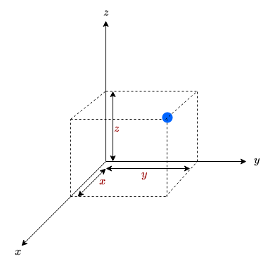
Figure 3: Coordinates in 3D |
Now about those Space Curves ...Consider the definition of a space curve. We see that, for any given value of $t$, we obtain an $x$, $y$ and $z$ value, the coordinates of a point lying on the space curve. Therefore, the single real input, $t$ produces a vector $(x,y,z)$, thereby lending the name vector-valued function. A vector-valued function is of the form $\overrightarrow{r{t}} = \left\langle f(t), g(t), h(t) \right\rangle$ where $f, g, h$ are real-valued functions of the parameter $t$. The path traced by a vector-valued function of such type is called a space curve. Consider the following rectangular coordinate equation given by $$\cos^{-1}{\frac{x}{a}} + \sin^{-1}{\frac{y}{a}} = \frac{2z}{c}$$ It is not immediately obvious how the plot of such a curve will look with a mere first glance. This is where parameterization becomes handy. The parametric equation of a helix is $$x = a \cos{t} \quad y = a \sin{t} \quad z = ct$$ As can be seen in Figure 2: as $t$ varies from $-\pi$ to $+\pi$, the curve is traced out. Parametrization in this case helps simplify the equation and makes the visualization process easirt. Sketching parametric curves can be done by eliminating the parameter, depending on the curve. Generally, one should exercise caution while plotting the points per various values of the parameter $t$, as the handful of points plotted may exclude details of the curve passing between any two points (as it is obviously not possible to plot all the points of the curve for the given range of the parameter!). Naturally, the first question which comes to mind while sketching a parametric curve by eliminating the parameter is: How do we eliminate the parameter $t$?
In mathematical terms, if $x = f(t)$ and $y = g(t)$ then we eliminate the parameter by setting $t = f^{-1}(x)$ and then using this value of $t$ inside $g(t)$ as $y = g(f^{-1}(x))$ However, this is not the most efficient way to eliminate the parameter. Why?
What we can do, however, is use various substitutions / trigonometric identities to eliminate the parameter. Note that we must find the limits enforced on $x$, $y$ and $z$ by the parametric curve to determine which portion of the algebraic curve is actually sketched via the parametric equations. Consider the example of the following parametric equation: $\quad x = \sqrt{r^{2} - u^{2}}\cos\theta \quad y = \sqrt{r^{2} - u^{2}}\sin\theta \quad z = u$ in the parameter interval $-1 \leq \sin\theta, \cos\theta \leq 1$ $\hspace{0.25cm} -1 \leq \sin\theta, \cos\theta \leq 1 \\ \implies -\sqrt{r^{2} - u^{2}} \leq \sqrt{r^{2} - u^{2}}\cos\theta, \sqrt{r^{2} - u^{2}}\sin\theta \leq \sqrt{r^{2} - u^{2}}$ $\hspace{0.1cm}\implies -\sqrt{r^{2} - u^{2}} \leq x,y \leq \sqrt{r^{2} - u^{2}}$ Hence, $x^{2} + y^{2} = 2(r^{2} - u^{2})$ which is the parametric equation of a circle. Hence, $x^{2} + y^{2} + z^{2} = 2r^{2} - u^{2}$, $u$ being a parameter. 0 |
|
0 |
|
Figure 4: Parametric circle to a sphere |
|
Let us take another example. A cone's parametric equations are given by: $$x = t \cos(t) \quad y = t \sin(t) \quad z = t$$ Eliminating the parameter $t$, we get: $$z^{2} = x^{2} + y^{2}$$ In the video given below, notice how the curve obtained describes the surface of the given cone. 1 |
|
2 |
|
Figure 5: Cone as a space curve |
Applications
HistoryIn 1749, D'Alembert submitted a memoir for a competition of the Berlin Academy on the resistance of fluids, involving three-dimensional fluid dynamics, which had only been a one-dimensional theory up to this point. Also, the upside-down model of churches by Antonio Gaudi was one of the earliest examples of parametric design. Pause and Ponder
References[1] https://colalg.math.csusb.edu/~devel/precalcdemo/param/src/param.html [2] http://www.it.hiof.no/~borres/j3d/math/param/p-param.html#maparam24 [3] https://ocw.mit.edu/courses/mathematics/18-02sc-multivariable-calculus-fall-2010/1.-vectors-and-matrices/part-c-parametric-equations-for-curves/session-17-general-parametric-equations-the-cycloid/MIT18_02SC_notes_9.pdfImages[4] Figure 3 has been generated using draw.ioFurther Reading[1] https://www.cs.helsinki.fi/group/goa/mallinnus/curves/curves.html [2] https://inst.eecs.berkeley.edu/~cs283/fa10/lectures/283-lecture19.pdf [3] http://web.cs.iastate.edu/~cs577/handouts/curves.pdf [4] https://www.math.miami.edu/~galloway/dgnotes/chpt2.pdf3 |
| Contributor: |
| Mentor & Editor: |
| Verified by: |
| Approved On: |
The following notes and their corrosponding animations were created by the above-mentioned contributor and are freely avilable under CC (by SA) licence. The source code for the said animations is avilable on GitHub and is licenced under the MIT licence.
