Partial Derivatives |
|---|
DefinitionThe partial derivative of $f(x, y)$ with respect to $x$ at the point $(x_0 , y_0)$ is $$\frac{\partial f}{\partial x} \vert_{(x_0 , y_0)} = \frac{d}{dx}f(x,y_0)\vert_{x=x_0} = \lim_{h \to 0} \frac{(x_0 + h,y_0)- f(x_0,y_0)}{h}$$ and with respect to $y$ at the point $(x_0 , y_0)$ is $$\frac{\partial f}{\partial y} \vert_{(x_0 , y_0)} = \frac{d}{dy}f(x_0,y)\vert_{y=y_0} = \lim_{h \to 0} \frac{f(x_0,y_0+ h)- f(x_0,y_0)}{h}$$ provided the limit exists.
-4 |
MotivationConsider the ideal gas law: $PV = nRT$ where $P$, $V$ and $T$ are the pressure, volume and temperature of the gas; and $R$ is the ideal gas constant. Suppose we want to observe the change in Volume ($V$) of gas, when we vary the Pressure ($P$) applied to it. The function is given as $V = f(n,P,T) = \frac{nRT}{P} = nRTP^{-1}$. But the ideal gas law equation contains another variable Temperature ($T$), so we can't find the change in $V$ with respect to $P$ directly. This can be done with partial derivatives by keeping another variable/s constant (in this case $T$) (http://homepages.wmich.edu/~dschreib/Courses/Chem637/RvPDff2.htm). Also consider a hill which can be viewed as the surface $z = f(x, y)$. The slopes from west to east ($x$-axis direction) and from south to north ($y$-axis direction) may be different and can be found from the concept of partial derivatives, which we will be looking further. -4 |
|
-3 |

Figure 1: Partial derivatives in Ideal Gas Law |
|
-3 |
|
Video 1: Slope of a hill along $X$ and $Y$ axis |
Bird's Eye ViewLet $f(x,y)$ be a function of two variables. The partial derivative of $f$ with respect to $x$ is obtained, if $y$ is kept constant and $f$ is differentiated with respect to the variable $x$, which is denoted by $$\frac{\partial f}{\partial x} \text{ or } f_x$$ Similarly, the partial derivative of $f$ with respect to $y$ is obtained, if $x$ kept constant and $f$ is differentiated with respect to the variable $y$, which is denoted by $$\frac{\partial f}{\partial y} \text{ or } f_y$$ The partial derivatives of $f(x, y)$ with respect to $x$ and $y$, at a point $(x_0, y_0)$ are denoted as $f_x(x_0, y_0)$ and $f_y(x_0, y_0)$ respectively. The partial derivatives are just like ordinary derivatives, except you keep any other variables constant (i.e. replacing these variables with their constant values). This rule is feasible for calculating partial derivatives because it reduces the matter just to compute the ordinary derivatives. -3 |
|
-3 |
|
Video 2: Partial Derivatives |
|
-2 |

|
Context of the Definition-1 |
|
0 |
|
Video 3: Partial Derivatives along $X$ and $Y$ axis |
|
In the video 3, the graph of a function $z= f(x,y) = 2-x^2 -y^2$ is a surface, and by fixing $y = b$ (Here $y = 0$) gives a curve (shown in green). The derivative measures the steepness of the graph of a function at some particular point on the graph (i.e. a ratio of change in the value of the function to change in the independent variable). Thus, the derivative is a slope. Since partial derivatives are just like ordinary derivatives except keeping any other variables constant. Therefore, the partial derivative $\frac{\partial}{\partial x} f(a,b)$ is the slope of the tangent line to the curve ($y = b$) at the point where $x=a$. Similarly, by fixing $x = a$ (Here $x = 0$) gives a curve (shown in dark blue). The partial derivative $\frac{\partial}{\partial y} f(a,b)$ is the slope of the tangent line to this curve at the point where $y=b$. Thus, the partial derivative $f_x(a,b)$ is the slope of the curve of $f(x,y)$ for the plane $y=b$ at the point $(a,b)$. Likewise the partial derivative $f_y(a,b)$ is the slope of the curve of $f(x,y)$ for the plane $x=a$ at the point $(a,b)$.
0 |
|
1 |
|
Video 4: Slope of Function at different $X$ and $Y$ values |
Partial Derivatives as FunctionsThe partial derivatives of functions of more than two independent variables are like the ordinary derivatives with respect to one variable, except all the other independent variables are held constant. In general, the partial derivative of a function of several variables $f(x_1,x_2, \cdots, x_m)$ with respect to some variable $x_i$, where $i \in 1,2, \cdots,m$ is denoted as $$f'_{x_i}(x_1,x_2, \cdots, x_m) = \frac{\partial }{\partial x_i}f(x_1,x_2, \cdots, x_m);$$ the symbol $\frac{\partial}{\partial x_i}$ means differentiation with respect to $x_i$ while substituting all other variables with their numerical value which is independent of $x_i$.
Example: If $x$, $y$, and $z$ are independent variables and $f(x, y, z) = x \sin( y + 2z)$, then partial differentiation of function $f$ with respect to $z$ is given as $$\frac{\partial f}{\partial z} = \frac{\partial f}{\partial z} [x \sin(y + 2z)] = x \frac{\partial f}{\partial z} \sin(y + 2z)$$$$=x \cos ( y + 2z)\frac{\partial f}{\partial z} ( y + 2z) = 2x \cos( y + 2z).$$ 1 |
Higher-Order Partial DerivativesThe partial derivatives of a function can be differentiated with respect to any variable, as they are functions of several variables. For example, all possible second partial derivatives for a function of two variables are $$\frac{\partial f}{\partial x} \rightarrow \frac{\partial }{\partial x} \frac{\partial f}{\partial x} = \frac{\partial^2 f}{\partial x^2}, \hspace{1cm} \hspace{1cm} \frac{\partial }{\partial y}\frac{\partial f}{\partial x} = \frac{\partial^2 f}{\partial y \partial x },$$$$\frac{\partial f}{\partial y} \rightarrow \frac{\partial }{\partial x} \frac{\partial f}{\partial y} = \frac{\partial^2 f}{\partial x \partial y}, \hspace{1cm} \frac{\partial }{\partial y}\frac{\partial f}{\partial y} = \frac{\partial^2 f}{\partial y^2}.$$ Brief notations for higher order partial derivatives used, for example, $$\frac{\partial^2 f}{\partial x^2} = (f'_x)'_x = f''_{xx}, \frac{\partial^2 f}{\partial x \partial y} = (f'_y)'_x = f''_{yx}$$ and similarly for $ f''_{yy}$ and $ f''_{xx}$. Similarly, the third-order partial derivatives can be seen as the partial derivatives of second-order partial derivatives, and so on. Example: Find all second and third-order partial derivatives for the function $f(x,y) = x^4 -x^2y + y^2$, . Solution: The first-order partial derivatives are $$f_x = 4x^3 - 2xy, f_y = -x^2 + 2y.$$ Then the second-order partial derivatives are $$f''_{xx} = (4x^3 - 2xy)'_x = 12x^2 - 2y, \hspace{1cm} f''_{yy} = (-x^2 +2y)'_y = 2,$$ $$f''_{xy} = (4x^3 - 2xy)'_y = -2x, \hspace{1cm} f''_{yx} = (-x^2 +2y)'_x = -2x.$$ The third-order partial derivatives are found similarly: $$f'''_{xxx} = (12x^2 -2y)'_x = 24x, \hspace{1cm} f'''_{yyy} = (2)'_y = 0,$$$$f'''_{xxy} = (12x^2 - 2y)'_y = -2, \hspace{1cm} f'''_{xyx} = f'''_{yxx} = (-2x)'_x = -2,$$$$f'''_{yyx} = (2)'_x = 0, \hspace{1cm} f'''_{yxy} = f'''_{xyy} = (-2x)'_y = 0.$$ The higher-order partial derivatives can be obtained by differentiating with respect to different variables in different orders, like $f''_{xy}$ and $f''_{yx}$. In the above example, it has been established that $$f''_{xy} = f''_{yx},$$$$f'''_{xxy} = f'''_{xyx} = f'''_{yxx},$$$$f'''_{xyy} = f'''_{yyx} = f'''_{yxy};$$ which means the result obtained from the various order in which the partial derivatives have been taken is independent of order . Is this an anomaly of the considered function or is it a general property of higher-order partial derivatives? The subsequent theorem answers this question. 1 |
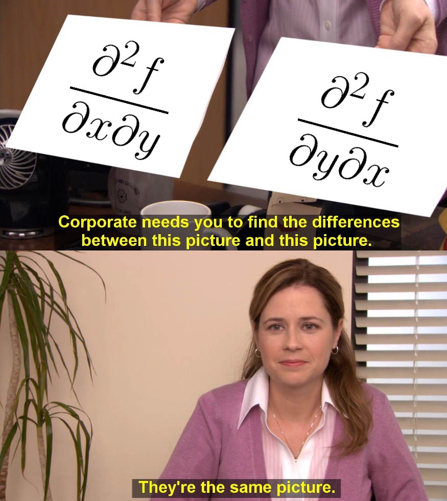
Clairaut’s TheoremConsider $f$ to be a function of several variables $(x_1, x_2, \cdots, x_m)$ defined on an open ball $D$. If the second-order partial derivatives $f''_{x_ix_j}$ and $f''_{x_jx_i}$, where $j \neq i$, are continuous functions on $D$, then $f''_{x_ix_j} = f''_{x_jx_i}$ at any point of $D$. Clairaut’s theorem result can be proved. It states that: The result of partial differentiation does not depend on the order in which the partial derivatives have been taken if all higher-order partial derivatives are continuous.
2 |
|
3 |

Figure 2: Mixed partial derivatives |
|
3 |
|
Video 5: Partial Derivative of a Function $z = (x^2 + 3y^2)e^{(1 - x^2 - y^2)}$ at $x = 0$ and $y = -1$ |
|
3 |

|
The Chain RuleThe Chain Rule for functions of a single variable states that when $w = f(x)$ is a differentiable function of $x$ and $x = g(t)$ is a differentiable function of $t$, $w$ is a differentiable function of $t$ and $\frac{dw}{dt}$ can be calculated as $$\frac{dw}{dt} = \frac{dw}{dx} \frac{dx}{dt}.$$ For this composite function $w(t) = f(g(t))$, we can think of $t$ as the independent variable and $x = g(t)$ as the “intermediate variable”, because $t$ determines the value of $x$ which in turn gives the value of $w$ from the function $f$. For functions of several variables, the Chain Rule has more than one form, which depends on how many independent and intermediate variables are involved. However, once the variables are taken into account, the Chain Rule works in the same way as discussed. 3 |
Chain Rule for Functions of One Independent Variable and Two Intermediate VariablesIf $w = f(x, y)$ is differentiable and if $x = x(t)$, $y = y(t)$ are differentiable functions of $t$, then the composite $w = f(x(t), y(t))$ is a differentiable function of $t$ and $$\frac{dw}{dt} = f_x(x(t),y(t))\cdot x'(t) + f_y(x(t),y(t))\cdot y'(t),$$ or $$\frac{dw}{dt} = \frac{\partial f}{\partial x} \frac{dx}{dt} + \frac{\partial f}{\partial y} \frac{dy}{dt}.$$ Proof: The proof consists of showing that if $x$ and $y$ are differentiable at $t = t_0$, then $w$ is differentiable at $t_0$ and $$\left( \frac{dw}{dt} \right)_{t_0} = \left( \frac{\partial w}{\partial x} \right)_{P_0} \left( \frac{dx}{dt} \right)_{t_0} + \left( \frac{\partial w}{\partial y} \right)_{P_0} \left( \frac{dy}{dt} \right)_{t_0},$$ where $P_0 = (x(t_0), y(t_0))$. The subscripts indicate where each of the derivatives is to be evaluated. Let $\Delta x$, $\Delta y$, and $\Delta w$ be the increments that result from changing $t$ from $t_0$ to $t_0 + \Delta t$. where $\epsilon_1, \epsilon_2 \rightarrow 0$ as $\Delta x, \Delta y \rightarrow 0$. To find $\frac{dw}{dt} $, we divide this equation through by $\Delta t$ and let $\Delta t$ approach zero. The division gives $$\frac{\Delta w}{\Delta t} = \left( \frac{\partial w}{\partial x} \right)_{P_0} \frac{\Delta x}{\Delta t} + \left( \frac{\partial w}{\partial y} \right)_{P_0} \frac{\Delta y}{\Delta t} + \epsilon_1\frac{\Delta x}{\Delta t} + \epsilon_2 \frac{\Delta y}{\Delta t}.$$ Letting $\Delta t$ approach zero gives $$\left( \frac{dw}{dt} \right)_{t_0} = \lim_{\Delta t \to 0}{\frac{\Delta w}{\Delta t}}$$ $$ = \left( \frac{\partial w}{\partial x} \right)_{P_0} \left( \frac{dx}{dt} \right)_{t_0} + \left( \frac{\partial w}{\partial y} \right)_{P_0} \left( \frac{dy}{dt} \right)_{t_0} + 0 \cdot \left( \frac{dx}{dt} \right)_{t_0} + 0 \cdot \left( \frac{dy}{dt} \right)_{t_0}.$$ Many a times we take down $\frac{\partial w}{\partial x} $ for the partial derivative $\frac{\partial f}{\partial x} $, so the Chain Rule can be re-written as $$\frac{dw}{dt} = \frac{\partial w}{\partial x} \frac{dx}{dt} + \frac{\partial w}{\partial y} \frac{dy}{dt}.$$ 3 |
|
5 |

Figure 3: Chain Rule For Functions of One Independent Variable and Two Intermediate Variables |
Chain Rule for Functions of One Independent Variable and Three Intermediate VariablesIf $w = f(x, y,z)$ is differentiable and $x$, $y$ and $z$ are differentiable functions of $t$, then $w$ is a differentiable function of $t$ and $$\frac{dw}{dt} = \frac{\partial w}{\partial x} \frac{dx}{dt} + \frac{\partial w}{\partial y} \frac{dy}{dt} + \frac{\partial w}{\partial z} \frac{dz}{dt}$$. Surprisingly, the chain rule is used in Backpropagation Algorithm of neural networks [https://ml-cheatsheet.readthedocs.io/en/latest/backpropagation.html]. 6 |
Applications
7 |
HistoryThe history of the very specialized topic of partial differential equations and partial differentiation and integration has not received adequate attention for the early period preceding Leonhard Euler's momentous contributions to this subject. The pre-Eulerian history of the partial processes of the calculus is difficult to trace, for the reason that there existed at that time no recognized symbolism nor technical phraseology which would distinguish the partial processes from the ordinary ones. The notation and logic of the partial differential or partial derivative was introduced in 1786 by French mathematician Adrien-Marie Legendre and later adopted by German mathematician Carl Jacobi in 1841. 7 |
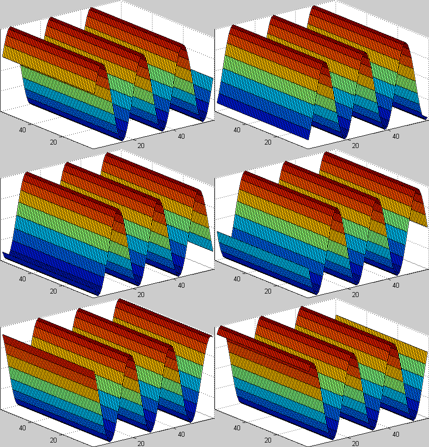
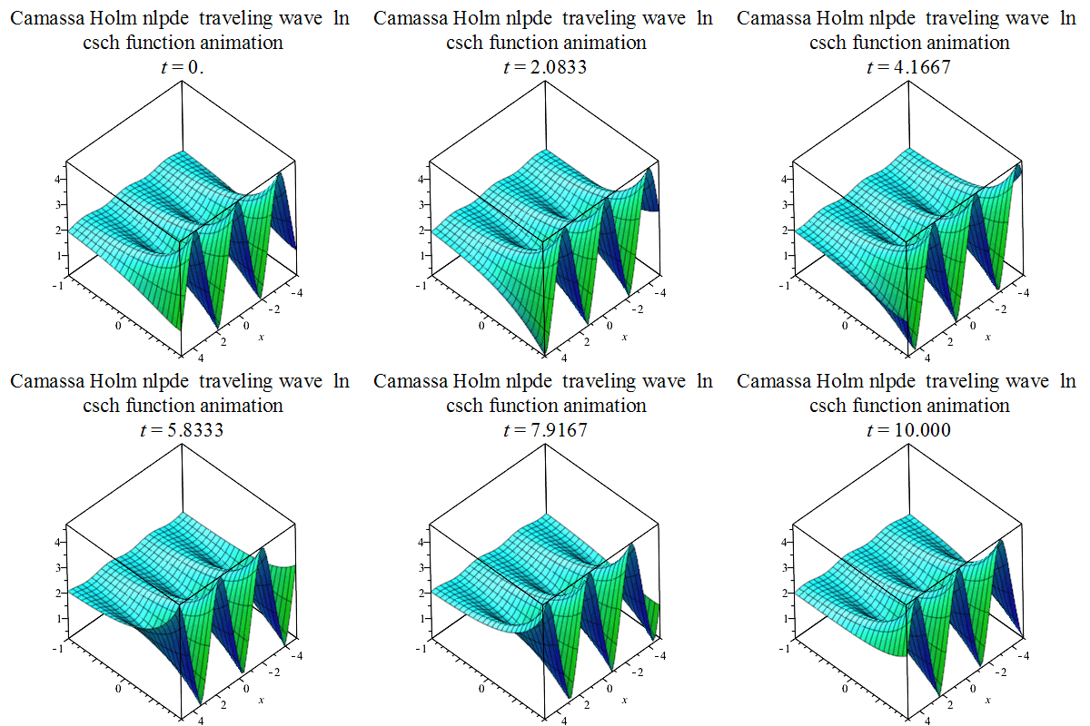
Pause and PonderThe relation between a function of several variables and its partial derivatives (of any order) is called a partial differential equation (PDE). Partial differential equations are a key tool to study various phenomena in nature. Many fundamental laws of nature can be stated in the form of partial differential equations. Partial differential equations occur in various areas of physics, chemistry, and engineering. There are different PDE examples, with their physical context like Diffusion Equation, Wave Equation, Laplace and Poisson Equations, etc. What is the role of the partial derivatives in the partial differential equations?
7 |
|
7 |

Figure 4: Plane Wave Travelling [2] |
|
7 |

Figure 5: Camassa Holm Equation Travelling Wave [3] |
References
7 |
Figures[2] Reproduced from https://commons.m.wikimedia.org/wiki/File:Camassa_Holm_equation_traveling_wave_csch_plot4.gif [3] Reproduced from https://commons.m.wikimedia.org/wiki/File:Plane_wave_animation.gif 7 |
| Contributor: |
| Mentor & Editor: |
| Verified by: |
| Approved On: |
The following notes and their corrosponding animations were created by the above-mentioned contributor and are freely avilable under CC (by SA) licence. The source code for the said animations is avilable on GitHub and is licenced under the MIT licence.
