Multivariable Functions |
|---|
DefinitionA multivariable function of $m$–variables is a function $ f : D \rightarrow \mathbb{R}^n$, where the domain $D$ is a subset of $\mathbb{R}^m$. So for each $(x_1, x_2, \cdots , x_m)$ in $D$, the value of $f$ is a is a real number $f(x_1, x_2, \cdots , x_n)$ called as scalar-valued function or a vector $f(x_1, x_2, \cdots , x_n) \in \mathbb{R}^n$ called as vector-valued function.
-2 |
MotivationThe density of an object could be found using a simple formula: $\text{Density}= \frac{\text{Mass}}{\text{Volume}}$. The density is a function of two variables Mass and Volume $f(\text{Mass}, \text{Volume})$. Likewise, the area of the box is a function of three variables, $\text{Area} = f(\text{Length}, \text{Breadth}, \text{Height}) = \text{Length} \times$ $\text{Breadth} \times \text{Height}$. These functions consists of multiple variables. Also, before designing any vehicle, it is first simulated on simulation software. Have you ever wondered how these vehicles, having different features, are simulated on the computer? The simple pendulum is modelled with many variables like length of rod L, a mass of bob m, and the angular position $\theta$ of the pendulum bob (with respect to vertical) which varies with time $t$. Thus the angular acceleration can be found, given as $\alpha = f(m,L, \theta)$ $= \frac{-b}{m}\omega - \frac{g}{L} \sin\theta$, where $\omega = \frac{d \theta}{dt}$. [https://services.math.duke.edu/education/ccp/materials/diffeq/pendulum/pend1.html] Similarly, different systems can be modelled having several parameters, which can be expressed as a function of several variables, called Multivariable Function. -2 |
|
-2 |
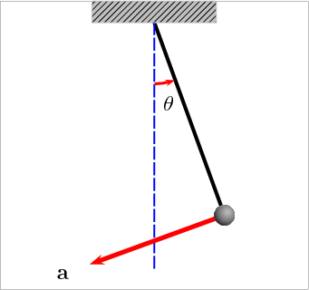
Figure 1: Simple Pendulum [1] |
|
-2 |
|
Video 1: Examples of Multivariable Functions |
Bird's Eye ViewIn general, a multivariable function is a function whose input consists of multiple numbers. $\displaystyle f(\!\!\!\!\!\!\! \underbrace{x,y,z,w}_{\substack{\text{Multiple numbers} \\ \text{in the input} }} \!\!\!\!\!\!\!) = x^3 y^2+ wz$ The output of a multivariable function consists of single or multiple numbers. If the output is a real-valued number, then the function is called a scalar-valued function, otherwise, it is called a vector-valued function, having vector as the output. -1 |
|
0 |
|
Video 2: Types of Multivariable Functions |
|
You can find more examples of multivariable functions in the lecture notes on <> Context of the DefinitionPoints in space $\Leftrightarrow$ List of numbersThe multivariable functions can be visualized as space having multiple dimensions. For example, let us consider a function that takes in two variables, like $(3, 5)$. Instead of thinking these inputs as two separate things, this can be taught as a single point in a two-dimensional space, with $x$-coordinate as 3 and $y$-coordinate as 5. Similarly, the three variable input $(3, 1, 2)$ can be taught as a single point in three-dimensional space instead of three separate things. So multivariable functions are about associating the points in one space with the points in some other space. For example, a function $f(x, y) = x^3 2y$, having two-variable input and a single-variable output, associates points in the $xy$-plane with the points on the number line. 0 |
|
0 |
|
Video 3: Multivariable Function in 3D Space |
Vector-Valued FunctionA vector, $f$, is called a vector-valued function of the vector variable $x$ if each of its $m$ components, $f_i$, are real-valued functions of $x$: $$f_i = f_i(x); f_i : \mathbb{R}^n \rightarrow \mathbb{R}, i = 1, 2,...,m$$ and $$f(x) = \langle f_1(x), f_2(x), \cdots ,f_m(x) \rangle$$
0 |
ExplanationWe say that $f : \mathbb{R}^n \rightarrow \mathbb{R}^m $ defines a transformation $x \rightarrow y = f(x): x_1, x_2, \cdots, x_n$ and $y_1 = f_1(x), y_2 = f_2(x), \cdots, y_m = f_m(x)$. The $f_i$, where $i = 1, 2, \cdots, m$, are the components of $f$ in the corresponding orthogonal directions $e_i$, where $i = 1, 2, \cdots, m$ in $\mathbb{R}^m$ (i.e., $i,j, k$ in $\mathbb{R}^3$). From this most general form, we now consider three important specific classes of vector-valued functions. Consider a point on a curve which is formed from a vector, from the origin to the point. As the point travels along the curve, the vector changes to terminate at the specified point. Thus, the curve can be taught as a collection of terminal points of vectors emanating from the origin. Accordingly, a point travelling along this curve can be seen as a function of time $t$, Therefore, we can define a function $r$, having input variable $t$ and spits a vector as the output, from the origin to the point on the curve at time $t$. As a result, a new type of function has been introduced, whose input is a scalar and the output is a vector. The output of the function $r$ is the vector from the origin to a point on the curve is defined by $r(t) = \langle x (t), y(t), z(t) \rangle$. Keep in mind that the input of $r$ is the real-valued parameter $t$ and the corresponding output is vector $\langle x (t), y(t), z(t)\rangle$. For example, let us consider the curve $C$ traced by the vector-valued function $\vec r (t) = \langle t,\pi \sin t \rangle, 0\leq t\leq 2\pi$. This vector valued function traces one period of the sine function . So the value at $\vec r (0)=\langle 0,0\rangle, \vec r (\frac{\pi}{2})=\langle \frac{\pi}{2},\pi \rangle, \vec r (\pi)=\langle \pi,0\rangle, $ and so on. The following video shows the curve $C$ and some position vectors. 0 |
|
1 |
|
Video 4: Vector Valued Function |
|
1 |
|
Video 5: Vector valued function in 3D space |
Differentiation of Vector-Valued FunctionThe derivative of a vector-valued function $\textbf{r}(t) = \langle x(t), y(t), z(t) \rangle$ with respect to $t$ is given by $$\textbf{r}'(t) = \frac{d}{dt}\textbf{r}(t)$$ $$= \frac{d}{dt} \langle x(t), y(t), z(t)\rangle$$ $$= \langle \frac{d}{dt}x(t), \frac{d}{dt}y(t), \frac{d}{dt}z(t)\rangle$$ $$= \langle x'(t), y'(t), z'(t)\rangle$$ assuming that the derivatives exist. Note that $\textbf{r}'(t)= \langle x'(t), y'(t), z'(t) \rangle$ is itself a vector-valued function. Visually, the vectors given by $r'(t)$ can be shifted in such a way that they are tangent to the curve traced out by $\textbf{r}(t) = \langle x(t), y(t), z(t) \rangle$. In a physical setting, if $\textbf{r}(t) = \langle x(t), y(t), z(t) \rangle$ represents the displacement of an object, then $v(t) = \textbf{r}'(t)= \langle x'(t), y'(t), z'(t) \rangle$ represents the object’s velocity and it's the magnitude, $|\textbf{r}'(t)|$, is the object’s speed. The object's acceleration is $a(t)=v'(t) = \textbf{r}''(t)= \langle x''(t), y''(t), z''(t) \rangle$. 1 |
|
1 |
|
Video 6: Differentiation of the Vector Valued Function |
Applications
1 |
|
4 |

Figure 2: The development of a cyclone depends on various factors like wind speed, wind direction, temperature, and humidity [2] |
HistoryMultivariable FunctionsDuring the $16^{th}$ century, mathematicians were developing new mathematics to tackle issues in physical science. Since the physical world is multidimensional, a significant number of these quantities utilized in these applied models were multivariable. Astronomy was one of the scientific areas which were rich in this sort of multivariable mathematics. Along these lines, the stage was being set by astronomers and mathematicians for the development of multivariable functions and multivariable calculus. Galileo (1564 - 1642) endeavored to apply mathematics to his work in astronomy and physics of kinematics. Johannes Kepler (1571 - 1630) contributed extraordinarily through the development of his three laws of planetary motion which helped discredit Ptolemy's geocentric model and built up Copernicus's heliocentric theory. It also set the stage for the rise of multivariable applied mathematics. After the development of single variable calculus in the 17th century, its application to problem-solving in the multidimensional world resulted in the need for generalization to include functions of more than one variable and multivariable calculus. 5 |
Pause and PonderIn Collaborative Filtering, a website/app tries to predict a user's behavior. It creates a function that takes in many variables such as the user's age, the coordinates of their location, the number of times they've clicked on links of a certain type, etc. The output might also include multiple variables, such as the probability that they will click on a different link or the probability they purchase a different item. [http://faculty.chas.uni.edu/~schafer/publications/CF_AdaptiveWeb_2006.pdf] Can you think of any other multivariable functions that are used in your daily life, but not be aware of it? 6 |
|
7 |
Figure 3: Collaborative Filtering [3] |
References
8 |
Figures[1] Reproduced from Ruryk / CC BY-SA (https://creativecommons.org/licenses/by-sa/3.0/), https://commons.wikimedia.org/wiki/File:Oscillating_pendulum.gif [2] Reproduced from https://upload.wikimedia.org/wikipedia/commons/thumb/a/a2/Marcia_Feb_20_2015_Landfall.gif/480px-Marcia_Feb_20_2015_Landfall.gif [3] Reproduced from Moshanin / CC BY-SA (https://creativecommons.org/licenses/by-sa/3.0/), https://commons.wikimedia.org/wiki/File:Collaborative_filtering.gif 9 |
| Contributor: |
| Mentor & Editor: |
| Verified by: |
| Approved On: |
The following notes and their corrosponding animations were created by the above-mentioned contributor and are freely avilable under CC (by SA) licence. The source code for the said animations is avilable on GitHub and is licenced under the MIT licence.
