The contents of this lecture notes are yet to be edited by mentors and get verified by a Professor.

Gradient

Definition

$\textrm{grad } f(x_0, y_0,z_0,...) = \nabla f(x_0, y_0,z_0,...) = \begin{bmatrix} \frac{\partial f}{\partial x}(x_0, y_0,z_0,...)\\ \frac{\partial f}{\partial y}(x_0, y_0,z_0,...)\\ \frac{\partial f}{\partial z}(x_0, y_0,z_0,...)\\ .\\ . \end{bmatrix}$

-1

Motivation

The gradient can be thought of as the multidimensional analogue of the one dimensional slope, given by the derivative. A popular preliminary example encountered while studying single variable calculus is that of the ball rolling down a hill. Notice how the calculation of the rate of change doesn't have to factor in the direction of the movement of the ball; since the hill itself is one dimensional, there is one direction (only one dependent variable in single variable functions) in which the ball can move. So is not the case when we move to higher dimensions. In higher dimensions (functions of several variables), the gradient takes the place of the derivative to calculate the slope.

Animation 1: The gradient is a multidimensional analogue of the derivative.

Since there are now more than a single path the ball can take down the hill, the slope of the hill would depend on the direction as well. The gradient, which accounts for the direction, gives the slope of the hill.

Bird's Eye View

The gradient, represented by the symbol nabla, $\nabla$ is an operator that calculates the rate of change of a function of more than one variable. Going back to the example of the hill, the gradient operator takes into consideration both the direction and position of the point at which the slope has to be calculated. Recall that while computing the slope of single variable functions, only the position had to be taken into account.

The gradient operator takes as input a function, and gives as output a vector field.

Animation 2: The gradient operator takes the function and gives a corresponding vector field

The specification of both position and direction is captured by the idea of partial differentiation. The rate of change of a multivariable function f(x,y) in the x direction is given by its partial derivative with respect to x, which is $\frac{\partial f}{\partial x}$. Similarly, $\frac{\partial f}{\partial y}$ represents the change of f in the y direction. The components of the vector field that $\nabla $ outputs are precisely these partial derivatives.

Animation 3: The process of computing the gradient

Context of the Definition

Why partial derivatives?

The formula of the gradient involves partial derivatives, one corresponding to each variable the function is defined over. Each partial derivative gives the rate of change of the function with respect to a particular variable. A vector field defined by a mix of these partial derivatives reflects their combined effect. The animation below clarifies this idea further.

Animation 4: Each point in the vector field has a vector attached to it, which represents the combined result of the rate of change of the function with respect to x and with respect to y.

Properties of the Gradient

Before beginning the exploration into the properties of gradients, let's look at contour plots.

A contour plot is a graph popular in topography and the study of inclines in landforms. Contour maps are used to indicate regions of constant altitude.

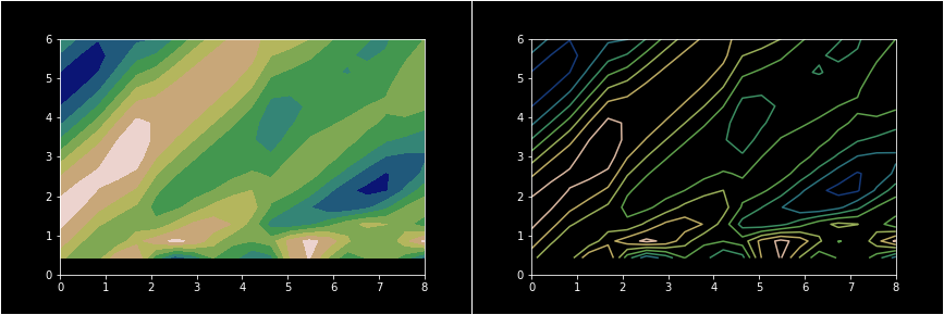
Figure 1: Contour maps are used widely in topography. It represents a three dimensional landform by plotting constant z slices onto a two dimensional surface.

1. The gradient at a particular point is perpendicular to any line of zero incline passing through that point

Each contour line indicates a constant z value. This is why it is also referred to a level curve has no incline. The rate of change of the function at any point on the level curve is zero, as $f(x,y)= c$. In other words, the value of its directional derivative, given by $\left\| \nabla f \right\|. cos\theta = 0$. Since the dot product is 0, we have that $\theta = 90$. Thus, the gradient is always perpendicular to the level curve.

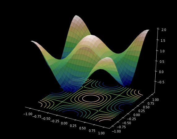
Figure 2: The figure shows how a three dimensional function is mapped onto a two dimensional contour plot.

Let's take a brief look at directional derivatives before moving on to the next property.

Directional derivatives

The directional derivative $\nabla_u f(x_0, y_0, z_0)$ is the rate at which the function $f(x,y,z)$ changes at a point (x_0, y_0, z_0) in the direction of a unit vector $\vec u$. It is computed using the formula

$\nabla_{\vec u} f = \nabla f \cdot \frac{\vec u}{\left | u \right |}$

Note: We do not go deeper into directional derivatives here as they have been covered in greater depth in a previous lecture

2. The gradient points in the direction of steepest ascent

Let $f(x, y) \textrm{be a function such that} f(x, y) = -(x^2 + y^2)$. How can we maximise $f_{\vec u}(x, y)$ at a point $x_0, y_0$? In other words, which unit vector maximises the directional derivative of f along $\hat u$?

To answer this question, consider the formula of the directional derivative

$\nabla_{\vec u} f = \nabla f \cdot \frac{\vec u}{\left | u \right |}$

$= \left | \nabla f \right | \left | u \right | cos \theta$, where $\theta$ is the angle between the gradient vector at $(x_0, y_0)$ and the unit vector $\hat u$

The dot product attains its maximum value when $cos \theta = 1$, or $\theta = 0$. Hence, the directional derivative is maximised when the unit vector points in the same direction as the gradient at that point, and therefore one can conclude that the gradient points in the direction of steepest ascent.

3. A zero gradient indicates a local maximum

The intuition for this property follows directly from the previous one. Since the gradient is an operator that points in the direction of greatest increase, a zero gradient would mean you are already at the point of greatest increase. Any movement from this point will result in a decrease in the output of the function f.

Applications

The gradient sees numerous applications in various fields of science and technology.

Predominantly used in physics, it is a foundational element in interpreting Maxwell's Equations that features in the fields of optics, electromagnetism, and electric circuitry.

In biology and life sciences, the gradient finds its application in a particular process by which motile cells move. Chemotaxis depends on the gradient of the relative concentration of the substance surrounding the cell.

In the field of population dynamics and evolution, the notion of a fitness function is used to determine the survival of a population of species. the increase or decrease of a population depending on various parameters, and is given by the gradient of the fitness function.

The derivative and the gradient are analogous The laws mentioned above are examples of $gradient$-driven transport.
Fick's First Law of Diffusion	built upon the concentration gradient	$f = -D \frac{\partial C}{\partial x}$
Ohm's Law	built upon the potential gradient	$i = -\sigma \frac{\partial V}{\partial x}$
Fourier's Law of Heat Transfer	built upon the thermal gradient	$h = -\lambda \frac{\partial T}{\partial x}$

Animation 7: A heat-seeking missile moves in the direction of greatest increase in temperature, which leads it most rapidly to the hottest part of the enemy aircraft - its engine. In this way, the heat-seeking missile makes use of a temperature gradient.

HISTORY

Physical mathematics is very largely the mathematics of $\nabla$.

Oliver Heaviside

It is widely believed that the formal study of vector calculus began in response to the need in the physical sciences, to describe forces and velocities. The notion of the gradient finds its thorough use in physics, and has historically been an integral tool in the physicist's inventory.

Devised by Hamilton during his study of quaternions, the symbol for the gradient, called nabla and denoted $\nabla$ comes from the Greek word for the Pheonician harp. It makes its appearance several times in letters exchanged between schoolmates Clerk Maxwell and Peter Tait. About a problem dealing with orthogonal planes, Maxwell wrote to Tait "It is neater and perhaps wiser to compose a nablody on this theme which is well suited for this species of composition." Maxwell dedicated his Tyndallic Ode to Tait, referring to him in it as the "Chief Musician upon Nabla".

PAUSE AND PONDER

(or wait and $\nabla$-iberate ? )

What does the gradient equal near the local minimum of a function?
The gradient takes in a scalar and outputs a vector. Can you think of an operator that takes in a vector to give a scalar, or takes in a vector to give another vector? What would such operators represent physically? (Hint: consider taking a dot product, or a cross product of the terms that define the gradient)
Is the gradient a linear operator? In other words, is it always true that "the gradient of a sum is equal to the sum of the gradients?"
The animation below portrays the flow of a fluid. Notice how it swirls. Is there a reason such a vector field cannot be the gradient of any function?

(Hint: The gradient points in the direction of steepest ascent)

Animation 8: Notice how the fluid swirls. Which is the direction of steepest ascent in this vector field?

References

Arfken, George B. Weber, Hans J. Harris, Frank E. Mathematical Methods for Physicists: A Comprehensive Guide. Academic Press, 2012 - p.143 - Chapter 3.5: Differential Vector Operators
Hubbard, John Hamal. Hubbard, Barbara Burke. Vector Calculus, Linear Algebra and Differential Forms: A Unified Approach. Matrix Additions, 2009 - p.627 to p.635 - Chapter 6: Forms and Vector Calculus
"The Gradient Vector", Math Insight, URL: https://mathinsight.org/gradient_vector
Stewart, James. Day, Troy. Biocalculus: Calculus, Probability, and Statistics for the Life Sciences. Cengage Learning, 2015 - p.610 to p.620 - Chapter 9.4: Directional Derivatives and the Gradient Vector

Contributor:

Mentor & Editor:

Verified by:

Approved On:

The following notes and their corrosponding animations were created by the above-mentioned contributor and are freely avilable under CC (by SA) licence. The source code for the said animations is avilable on GitHub and is licenced under the MIT licence.