Double Integrals |
|---|
DefinitionIf we have a well behaved function [1] $f(x,y)$ in a region $R$ then the double integral in that region is defined as --
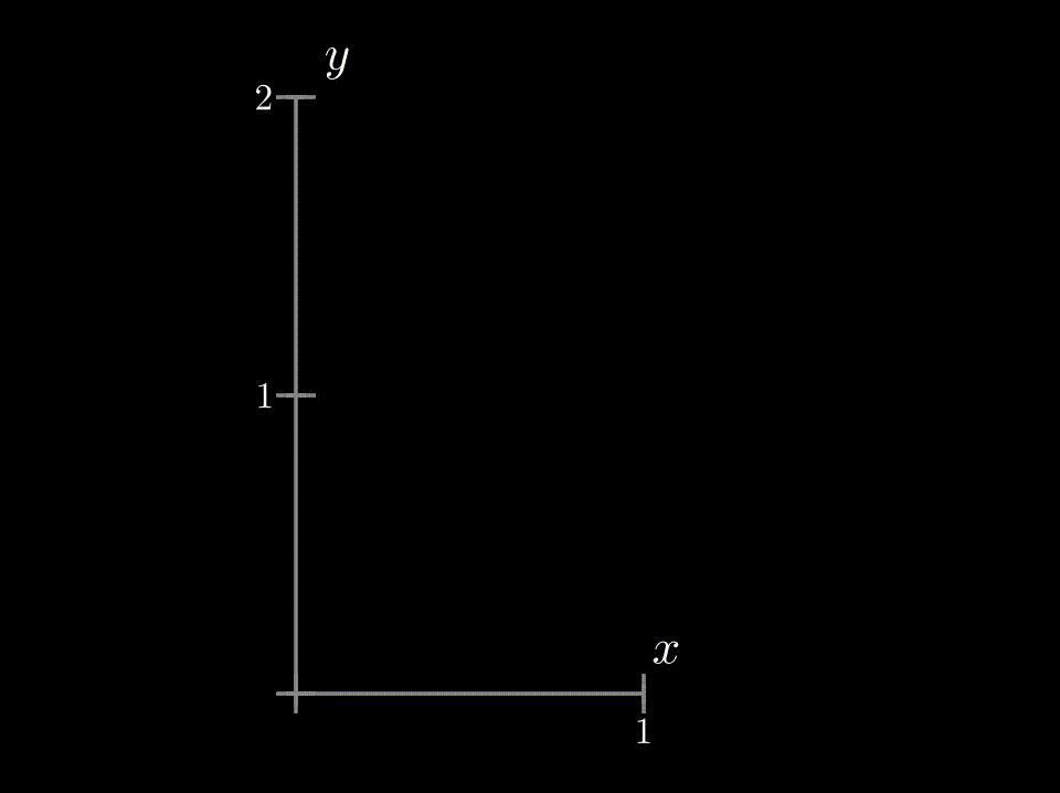
$$\int\int_{R} f(x,y)\ dA$$ Where $dA$ is the elementary area in the region $R$. Generally, double integral of the function $f(x,y)$ is beautifully defined as the limit of Riemann sums[2] in the region $R$ -- $$\lim_{n \to \infty}\sum_{i=1}^{n} f(x_i,y_i)\ \Delta A_i$$ Where, the region $R$ is divided into n small regions , i-th element having area $\Delta A_i$ and in that element at some point $(x_i,y_i)$ the function has the value $f(x_i,y_i)$.
-1 |
MotivationWe have been using integration for finding area, mass, the moment of inertia, and so on. The use case of integration is indispensable. And as we jump into the realms of functions with more than one variable, it is natural to ponder on how integration - as a process - will evolve. Double Integral is the first step towards Multiple Integral, which has immense applications in probability theory, Turbulent Flows, improvement of combustion engines, and more in engineering and architecture [3]. In single variable calculus, typically we thought of integration as the area under the curve - similarly, building up to the same analogy, we'll see how the double integral can be interpreted as the volume under a surface. -1 |
Bird's Eye ViewA single variable function $f(x)$ can be represented as a curve in X-Y plane. For $f(x)$ the definite integral $\int_{a}^{b} f(x) dx$ represents area under the curve between $a\leq x \leq b$ . -1 |
|
-1 |
|
Animation 1 : $\int f(x) dx$ is the area under the curve $y=f(x)$ and it can be represented as Riemann sum of infinitesimally thin rectangular areas. |
|
For function $f(x,y)$ the double integral $\int_{a}^{b}\int_{c}^{d} f(x,y)\ dx dy$ represent a volume under the surface in the region $R$ bounded by limits $a\leq x \leq b$ and $c\leq y \leq d$. 0 |
|
0 |
|
Animation 2: $\iint f(x,y)\,dxdy$ is the volume under the surface $z=f(x,y)$ and it can be approximated as sum of volume of cubiods. |
|
Usually, we use the integration formulas [5] to integrate a function but sometimes we encounter some stubborn functions which we cannot integrate by any method using the formulas. There comes the Riemann's sum method which is applicable in any situation, and it is based on calculating the area or volume by dividing the region into infinitesimal elements, but this is a numerical approach - we need computational power and it is quite straightforward.
For doing double integrals by non-numerical methods with help of anti-derivative formulas[5](i.e.$\int x^n dx= x^{n+1}/(n+1)$ ) we first set one of the variables (Let $y$) as a spectator and do the integration over the other variable (here $x$). Then we do the integration over $y$ as if we are collecting that "thick" areas along $y$, to get the whole volume under the surface of the function in the integration region. This is called the iteration method. 0 |
|
0 |
|
Animation 3 : Double integration process of the function $z=f(x,y)$ in the region $R$ |
Context of the DefinitionTo get the taste of it let's start with a function $f(x,y)=1+x+y $ to be integrated in the limit $0\leq x\leq 1 , 0\leq y\leq 2$. For the sake of seeing it in our coordinate system, we assign $z=f(x,y)$. To make it more meaningful (remembering the Riemann Sum), we restate the problem as - Find the volume of the region bounded by the planes $z=1+x+y,\ y=2,\ x=1$ and coordinate planes. $$\int_{x=0}^{1}\int_{y=0}^{2}(1+x+y)\ dydx$$ Let's first integrate over $y$ treating $x$ as some constant (process called iterated integration) -- $$\int_{x=0}^{1}\left(y+xy+\dfrac{y^2}{2}\right)\Bigg|_{0}^{2}\ dx = \int_{x=0}^{1}(4+2x)\ dx$$ The function $(4+2x)$ gives the area under the surface at some arbitrary $x$, and multiplied by $dx$ it gives a thin "slab" like volume! Now if we sum over all such "slabs" we will get the total volume; to do it we just have to integrate over $x$ . $$\int_{0}^{1}(4+2x)\ dx = (4x+x^2)\bigg|_{0}^{1} =5 $$ 0 |
|
0 |
|
Animation 4: Integration process of $z=(1+x+y)$ in the previous example. |
♦ Properties of the Double Integral
♦ Integration in non-rectangular regionsThe recipe given before is incomplete because we do not always have so nice constant values as limits, creating a rectangular region. Setting the limits for non-rectangular regions can be quite tricky. In those cases, it is best to draw the region and see what curves bound the region and serve as limits of integration. Lets see it with an example - again we choose the function $f(x,y)=(1+x+y)$ but now we have to get the volume of the region bounded by $z=f(x,y)$, $2x+y=2$ plane and coordinate planes . At first, we integrate over $y$, but we have to be cautious about the limit, as at different $x$ values the limit of $y$ is not a constant rather it is a function of $x$ $\rightarrow y=2-2x$. So here the integral becomes-- 0 |
|
0 |
The limit of $y$ is dependent on $x$ |
|
Evaluating the integral- Now if we have wanted to do the $x$ integral first then the setup would have been like- and one can verify that it also gives the same answer. Generally, the limits can be any function rather than being a straight line(For more see Ref:[6]). In those cases, it is best to draw the region and choose whether the $x$ integration or the $y$ integration should be done first! Choosing the integration order wisely can reduce the amount of work significantly and occasionally it happens that the function can't be integrated in the other way. Property 3. is also a useful tool. In some cases, it may happen that the boundary can't be expressed as a single function but we can divide the region to get some good functions. In real-life applications we have to approximate a region with some functions -- functions are not ready-made. 0 |
|
0 |
|
Integrating over non-rectengular region and division of the region to get some meaningful functions |
♦ Using the Polar Coordinate SystemSo far we used Cartesian Coordinate systems ( X-Y axis perpendicular on each other) but we can use any coordinate systems as feasible to the given problem. One of such most used coordinate system is polar coordinates. Probably you have noticed, "$dA$" used in the definition was substituted by "$dy\ dx$" in the previous examples. It is that because in Cartesian coordinate systems elementary area is a rectangle with sides "$dx$" and "$dy$". Similarly, we can find that in polar coordinates the elementary area is "$r\ dr\ d\theta$". 0 |
|
0 |
Elementary area expressed in rectangular and polar coordinates in a region. |
|
Let's see with an example how polar coordinates can be used for integration-- We again choose $f(x,y)=1+x+y$ and now we have to find the volume of the region bounded by $z=f(x,y)$ , $x^2+y^2=1$ and coordinate planes. In the spirit of previous sections the integral should be-- So we transform everything to polar coordinates, $f(x,y)\rightarrow f(r,\theta)=1+r(\cos\theta+\sin\theta)$, $dxdy\rightarrow r\ dr\ d\theta$. For setting the limits it is better to draw/imagine the region. 0 |
|
So in polar coordinates the integral becomes-- So, if you find some rotational symmetry try to use polar coordinates to evaluate the integral; it is not guaranteed that this will simplify the problem in every situation. ApplicationsWe have already seen that using double integral we can calculate the volume of a region. Next we calculate center of mass($\overline x,\overline y$) of a laminar object with mass density $\rho(x,y)=1+y$ and sides $y=0, y=x\ [0\leq x\leq2], y=(6-2x)\ [2\leq x \leq 3]$. \begin{align}M=\int dm &=\int\int\rho dA\\ &=\int_{0}^{2}\int_{0}^{x}(1+y)dydx+\int_{2}^{3}\int_{0}^{6-2x}(1+y)dydx\\ &=\int_{0}^{2}(x+\dfrac{x^2}{2})dx+\int_{2}^{3}((6-2x)+\dfrac{(6-2x)^2}{2})dx\\ &=5\end{align} \begin{align}\overline x &=\dfrac{1}{M}\int_{x=0}^{3}\int_{y=0}^{f(x)}x(1+y) dydx\\ &=\dfrac{1}{M}\left[\int_{0}^{2}\int_{0}^{x}x(1+y) dydx+\int_{2}^{3}\int_{0}^{6-2x}x(1+y) dydx\right] \\ &=\dfrac{1}{5}\left(\dfrac{14}{3}+\dfrac{23}{6}\right) \\ &=1.7\end{align}
0 |
|
0 |
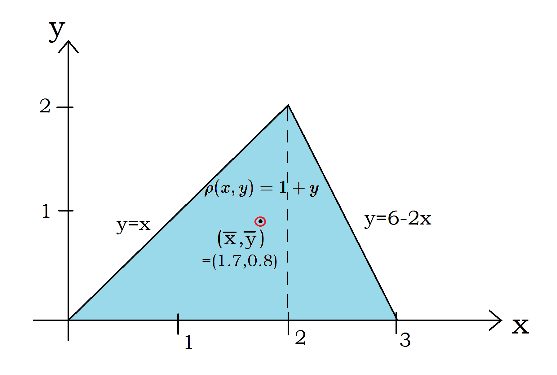
The center of mass of the laminar object in the example |
|
Do the integrals to get the answers by yourself? So we get the center of mass of the given lamina at $(\bar x=1.7,\bar y=0.8)$. It is an averaging process where elementary masses are multiplied by its distance from the axes. In a similar fashion, we can do statistical and probability calculations.(See Ref:[3] ,page-362 and Ref:[8]) In the calculation of surface integrals, double integral is the tool. 0 |
HistoryThroughout the 17th and 18th centuries Mathematicians were coming closer to the idea of Riemannian Integration and in the 19th century after the discovery of limits Cauchy first tried to make integral calculus more meaningful. Next in 1854 Riemann Integration came from Riemann's paper on trigonometric series. Gaston Darboux made the idea more clear & modified by defining the convergence of the Upper Riemann and Lower Riemann sums but then Dirichlet showed that not all functions are Riemann integrable. In this situation, Lebesgue introduced an alternative form of integration in 1902. Lebesgue's summarized his idea in a letter to Paul Montel:
Lebesgue's work is completely abstract and showed that Mathematics has marched far from merely being a tool for science. 0 |
Pause and PonderThink that integration is nothing but the sum of the values of the function at different points multiplied with the small areas/line-segments where the points reside. To do that by hand we have a shortcut (powered by calculus) --the antiderivative formulas. How can we think about the geometric interpretation of double integrals in Cylindrical Coordinates (or any other non-euclidean coordinate system)? 0 |
References
0 |
Further Reading
0 |
| Contributor: |
| Mentor & Editor: |
| Verified by: |
| Approved On: |
The following notes and their corrosponding animations were created by the above-mentioned contributor and are freely avilable under CC (by SA) licence. The source code for the said animations is avilable on GitHub and is licenced under the MIT licence.
