$\vec F$ is conservative $\implies$ curl $\vec F = 0$ |
|---|
Theorem
If $\vec F$ is a conservative vector field, then curl $\vec F = 0$
1 |
MotivationImagine rowing a boat inside a whirlpool. You don't have to expend energy doing physical work in order to increase your speed; the velocity of fluid flow increases as you move closer to the centre of the whirlpool. Would you say the velocity field of the whirlpool resembles a conservative field or a non-conservative one? Another associated property of the whirlpool is its curl. What is the nature of the curl of the whirlpool? What is the relationship between its curl and its conservative property?
2 |
|
3 |
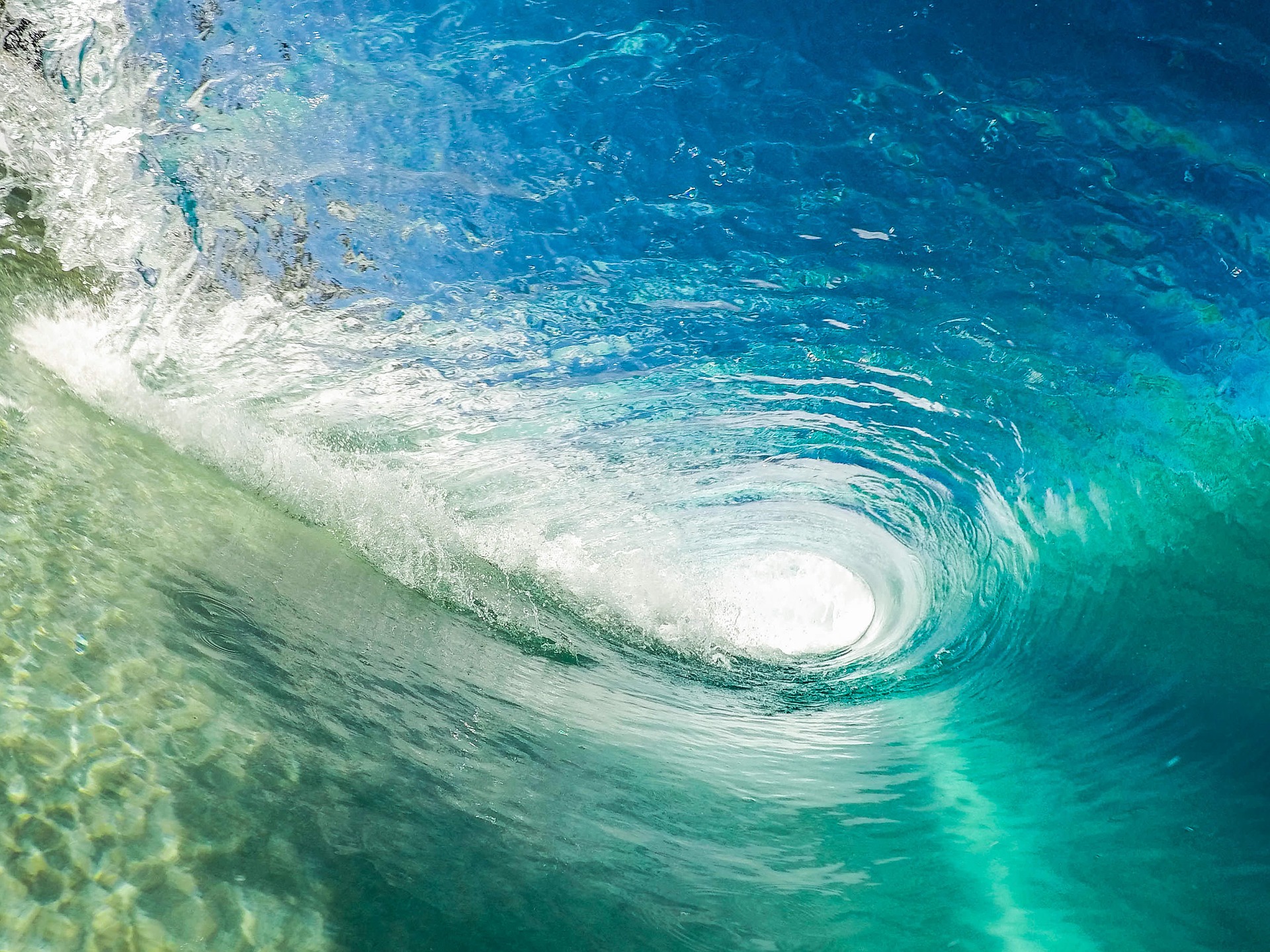
Figure 1: A whirlpool |
Bird's Eye ViewIn our discussion regarding conservative vector fields in the previous lecture, one aspect was strikingly absent. What is the nature of the curl associated with a conservative vector field? We know that the curl of a vector field indicates the degree of rotation of the vector field. Picture moving along an arbitrary circular path around the vector field. The total work done in going one round depends on the instantaneous rotation, or curl of the vector field. For a vector field that is conservative, the curl is zero. Conversely, for a field that is non-conservative, we obtain a non-zero curl. Why is this so? Additionally, can there exist vector fields which are seemingly conservative, but possess a non-zero curl? These questions are dealt with in the following sections. 4 |
|
5 |
|
Animation 1: Work done along a closed loop in a conservative field is zero |
Context of the Definition"If $\vec F$ is conservative, it implies that curl $\vec F = 0$ " The statement of the theorem deals with a couple of concepts we have encountered in the past. Let's do a quick review of them. The curl of a vector fieldCurl can be thought of as an operator that takes in one vector field and spits out another, The resultant vector field gives us an idea about the instantaneous rotation at a point in the vector field.
6 |
|
7 |
|
Animation 2: Recall from the lecture on curl, how a metaphorical paddle wheel is used to determine the components of curl |
The relationship between the curl and the line integralThe curl of a vector field is given by $\nabla \times \vec F$. The line integral of a vector field is computed using $\oint \vec F \cdot \vec dr$. What's interesting is that both the curl operator and the line integral are measuring the same thing - the circulation of the vector field. In certain cases, it might be more accurate to suggest that the curl measures the microscopic circulation at a particular point (or the limit of the region), while the line integral measures the macroscopic circulation along a curve. 8 |
|
9 |
|
Animation 3: Both the line integral and the curl operator can be used to measure circulation |
Conservative fieldsAs discussed in the previous lecture note, the conservative field is a vector field in which the line integral along a curve is path independent. Physically, this indicates that the work done in the field is dependent only on the end points and not the path that is taken. This also implies that a conservative field has zero curl, whereas going around a non-conservative field would give you some value of curl. Recall also, that if a field is conservative, it is also the gradient of some scalar function. In that sense, the words "conservative field" and "gradient field" are synonymous.
10 |
|
Equipped with these two concepts, we attempt to answer the following question - What is the curl of a gradient field?Let F be a vector field of the form $\vec F = \vec P\hat i + \vec Q\hat j + \vec R\hat k$ $\vec F$ may be written as the gradient of function f if the line integral $\oint_{C} \vec F \cdot \vec dr$ along a curve C is independent of its path. Hence, $\vec F = \nabla f$ That brings us to the theorem in consideration - Theorem: If $\vec F = \nabla f$, curl $\vec F = 0$ Proof: Since $\vec F = \nabla f$, $\vec F = \left \langle \frac{\partial f}{\partial x}, \frac{\partial f}{\partial y}, \frac{\partial f}{\partial z} \right \rangle$ Curl is calculated using the cross product notation $\begin{vmatrix} $= (\frac{\partial^{2} f}{\partial y \partial z} - \frac{\partial^{2} f}{\partial z \partial y} ) \hat i - (\frac{\partial^{2} f}{\partial x \partial z} - \frac{\partial^{2} f}{\partial z \partial x} ) \hat j + (\frac{\partial^{2} f}{\partial x \partial y} - \frac{\partial^{2} f}{\partial y \partial x} ) \hat k $ = 0 Note: The above results derives from Clairuat's Theorem, which speaks about the symmetry of second derivatives. This is why each component reduces to zero. We have successfully proved that the curl of a conservative field is zero. The converse of this theorem proposes is equally interesting; if the curl of the field is zero, does it imply that the field is conservative? Is curl $\vec F = 0$ a necessary condition for $\vec F$ to be conservative?
Necessary, but not sufficientConsider a vector field $\vec F$ with curl $\vec F = 0$. The circulation around a closed loop in this field is equal to zero. In other words, for a curve that begins and ends at the same point A, $\oint_{C} \vec F \cdot \vec dr = f(A) - f(A) = 0$ As discussed in the previous lecture, this is one of the properties of a conservative field. We may conclude that a vanishing curl is a necessary condition for the vector field to be considered conservative. However, this condition is not sufficient. We will see why using an example.
11 |
|
Example 1: Consider the vector field, $\vec F = \frac{1}{x^2 + y^2} \begin{bmatrix} popularly known as the vortex vector field. The vortex vector field resembles a whirlpool, which was used as an example in the Motivation section. curl $\vec F = \begin{bmatrix} $= \frac{(x^2 + y^2) -2x^2}{(x^2 + y^2)^2} + \frac{(x^2 + y^2) -2y^2}{(x^2 + y^2)^2}$ = 0 Given curl $\vec F = 0$, we should be able to write $\vec F = \nabla f$ for some function f. However, this is not possible, as we will see below. Consider a circle in the vector field, $g(t) = \begin{pmatrix} The work done along the circle oriented counter-clockwise is $\int \vec F \cdot \vec dr = \int_{0}^{2 \pi} \vec F (g(t)) \cdot g'(t) dt $ $ = \int \vec F \cdot \vec dr = \int_{0}^{2 \pi} \frac{1}{cos^{2} t + sin^{2} t} = $2 \pi$ For a conservative field, the work done around a closed path must be zero. Clearly, that is not the case above. We have found a vector field F with vanishing curl, which is not conservative. We cannot write $\vec F = \nabla f$, since $\vec F$ is not conservative. This conclusion is not very consistent, as the curl of the vector field is still 0.
A work-around - There is one way in which $\vec F$ can be represented as a gradient field. Check $\vec F = \nabla (arctan \frac{y}{x})$ This equation satisfies the condition above. How is this possible?
13 |
|
14 |
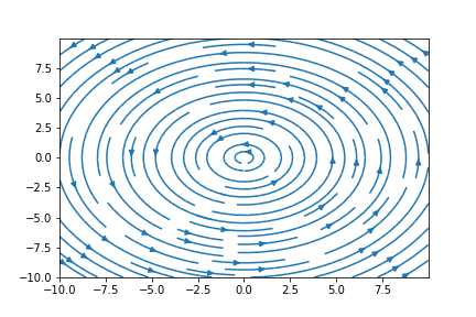
Figure 3: Streamplot of the vortex vector field |
Connected RegionsWith regards to the example taken above, the reason the line integration of $\vec F = \nabla (arctan \frac{y}{x})$ gives $2\pi$ despite having a vanishing curl is that f cannot be considered a function at all. In other words, the domain of f has holes in it when it is defined on $U = \left\{(x,y) \neq (0,0) \right\}$. If we restrict the domain of f such that the vector field is defined on the set $U' =\left\{x > 0 \right\}$ instead, the vector field has a corresponding potential function $ f = arctan(\frac{y}{x})$ In geometrical terms, U' is simply connected, whereas U is not. The formal definition of the term simply connected is given below -
Simply Connected: A region is simply connected if one can connect any two points in the region with a path and every path in the region can be deformed to a point within the region.
15 |
|
16 |
|
```````````````````````````````````````````````````Animation 4: Examples of simply connected regions |
|
17 |
|
Animation 5: Examples of regions that are not simply connected |
Pause and PonderIn the movie A Beautiful Mind based on the life of American mathematician John Nash, Nash challenges his class to a problem in vector calculus in which the region is not simply connected - Find a region X of $R^3$ with the property that if
V is the set of vector fields F on $R^3$/X which satisfy curl(F) = 0 and, W is the set of vector fields F which are conservative: $F = \nabla f$, then, the space $V/W$ should be 8 dimensional.
Although in the movie, Nash hopes the given problem will take his students the rest of their natural lives to solve it, giving it some thought is sure to bring us valuable insights. 18 |
|
19 |
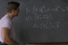
Figure 3: Still from $\textit{A Beautiful Mind}$ |
Further Reading
References
20 |
| Contributor: |
| Mentor & Editor: |
| Verified by: |
| Approved On: |
The following notes and their corrosponding animations were created by the above-mentioned contributor and are freely avilable under CC (by SA) licence. The source code for the said animations is avilable on GitHub and is licenced under the MIT licence.
