Curl and Divergence |
|---|
DefinitionsThe Del Operator, $\nabla$, is defined as $\nabla = (\frac{\partial }{\partial x},\frac{\partial }{\partial y},\frac{\partial }{\partial z})$.
For a vector valued function given by $\vec F = P\hat i + Q\hat j + R\hat k, $ we define Divergence as the dot product of $\nabla$ and $F$ $\textrm{div } \vec F = \nabla . \vec F = \frac{\partial P}{\partial x} + \frac{\partial Q}{\partial y} + \frac{\partial R}{\partial z}$ and Curl as the cross product of $\nabla$ and $F$ $\textrm{curl } \vec F = \nabla \times \vec F = \text{det}\begin{bmatrix} \hat{i}&\hat{j}&\hat{k}\\ \dfrac{\partial }{\partial x}&\dfrac{\partial }{\partial y}&\dfrac{\partial }{\partial z}\\ P&Q&R \end{bmatrix} = \left ( \frac{\partial R}{\partial y} - \frac{\partial Q}{\partial z} \right) \hat i + \left ( \frac{\partial P}{\partial z} - \frac{\partial R}{\partial x} \right) \hat j + \left ( \frac{\partial Q}{\partial x} - \frac{\partial P}{\partial y} \right) \hat k$
MotivationPicture a flowing river. In certain regions, it seems as though the water flows out from a point, while it simultaneously drains into some other points. As it forms vortices, it circulates faster in some places compared to others. You could say that the river appears to diverge and curl as it flows. This fluid flow metaphor, when extended to concepts in electromagnetism and fluid mechanics, facilitates an intuitive grasp of the div and curl operators. Therefore, will proceed by taking up examples of vector fields that represent the flow of fluid and try to understand div and curl in that context. 0 |
|
0 |
|
Animation 1: Fluid flow is an efficient metaphor to convey the meanings of divergence and curl. Div and curl can be used to describe the flow of water, primarily, and even the flow of filedlines in electromagnetism, the flow of air around planes in aerodynamics, and the flow of wind in weather maps. |
Bird's Eye ViewThe divergence of a field is captured by its source or sink-like behaviour. Similarly, curl talks about the rotation in the field.
0 |
|
0 |
|
Animation 2: Fluid flow illustrates divergence and curl |
|
1 |
|
Animation 3: Classification of divergence and curl |
|
The animation above illustrates the different types of two-dimensional divergence and curl. Divergence can be understood as a fluid's tendency to flow outwards or inwards. Positive divergence is characterised by source-like behaviour, similar to what you would see if you observed water shooting out from a hose. Negative divergence is characterised by sink-like behaviour, similar to what you would see if you looked at water flowing into a drain. Curl, on the other hand, measures the instantaneous rotation of the flow. In two dimensions, clockwise rotation indicates negative curl and vice versa. However, curl is generally applicable to three-dimensional vector fields. Suppose you curl the fingers of your right hand in the anti-clockwise direction, the direction of curl will be along your thumb, which points towards you. Notice how this is a direct application of the Right-Hand Thumb Rule. This connection is further strengthened when we take a look at the formula for curl, which involves taking the cross product. The three animations that follow show a three-dimensional vector field and its corresponding curl vector, as well as a three-dimensional vector field with negative divergence. 2 |
|
3 |
|
Animation 4: The vector field $\vec F = \left ( y^{3} - 9y \right) \hat i + \left ( x^{3} - 9x\right) \hat j + 0\hat k $ |
|
4 |
|
Animation 5: The resultant curl vector, $\vec G = 0\hat i + 0\hat j + \left( 3x^{2} - 3y^{2} \right) \hat k$ |
|
Three dimensional divergence is comparatively straightforward. The animation below shows negative divergence in three dimensions. 4 |
|
5 |
|
Animation 6: Negative divergence in three dimensions |
Macroscopic versus Microscopic CirculationThe curl operator that has just been introduced is a measure of a vector field's microscopic circulation, which is different from macroscopic circulation. This subtlety seems inconsequential, but is not, as is seen in certain cases. The microscopic curl of a vector field is a property of an individual point, not a region (more on this later). Take for example the ball shown in the animation below. Notice how while measuring microscopic curl, the centre of the ball is fixed, and the ball rotates around its axis. 6 |
|
7 |
|
Animation 7: Microscopic curl vs macroscopic curl |
Context of the DefinitionBreakdown of the formulas for Div and Curl:
Multivariable calculus, and in it the concepts of divergence and curl particularly, are often studied and understood for their applications in describing physical phenomenon. Nonetheless, an intuition for the concepts which is purely analytical is easily developed by starting with one of the most fundamental objects in vector calculus - the vector field. Consider a two dimensional vector field F, with components $F_{x}$ and $F_{y}$, dependent on x,y. Information about the rate of change of this field can be derived from the partial derivatives of F. $\frac{\partial F_{x}}{\partial x}$
$\frac{\partial F_{y}}{\partial y}$ $\frac{\partial F_{x}}{\partial y}$ $\frac{\partial F_{y}}{\partial x}$
Divergence
The divergence operator inputs a vector field and outputs a scalar value. The formula includes $\frac{\partial F_{x}}{\partial x}$ and $\frac{\partial F_{y}}{\partial y}$. $\frac{\partial F_{x}}{\partial x}$ describes the change in the horizontal component $F_{x}$ of $F$ at point $( x,y)$ in the $x$ direction. Similarly, $\frac{\partial F_{y}}{\partial y}$ measures the change in the vertical component $F_{x}$ of the vector field $F$ in the $y$ direction. The sum of these two partials, which is a scalar, gives the overall change of the vector fied at a point. To generalise divergence to three dimensions is simple; the sum would consist of the additional $\frac{\partial F_{z}}{\partial z}$ term.
7 |
|
8 |
|
Animation 8: The intuition for formula for divergence |
CurlCurl, unlike the divergence operator, takes in a vector field and outputs another vector field. The formula of curl considers the cross interactions - the partials $\frac{\partial F_{x}}{\partial y}$ and $\frac{\partial F_{y}}{\partial x}$. $\frac{\partial F_{x}}{\partial y}$ measures the change in the horizontal component as y changes, and $\frac{\partial F_{y}}{\partial x}$ measures the change in the vertical component as x changes. The measurement of the x component in terms of y and vice versa describes the rotation of each component. Consequently, the difference between the two partials represents the rotation of the vector field itself. This essentially is the 2D curl of the vector field. Three-dimensional curl, which is what captures the true essence of the operator, is computed differently. The $x,y,z$ axes have two cross interactions to consider each. In order to simplify this, imagine a paddle wheel inserted in at some point into a body of flowing fluid. The speed with which the paddle rotates is proportional to the component of the curl in the direction of the axle. 9 |
|
11 |
|
Animation 9: The paddlewheel analogy to compute three dimensional curl with respect to each component |
Formal definitions of div and curl
$div F(x,y) = \lim_{A_{x,y} \to 0}( \frac{1}{A_{x,y}} \oint_{C}\vec F \cdot n\hat ds )$
$curl F(x, y) = \lim_{A _{x,y} \to 0}( \frac{1}{A_{x,y}} \oint_{C}\vec F \cdot dr) $ Note: The purpose of this section is not to elaborate on the formal definitions as much as talk about why these formal definitions are necessary.
Divergence represents the "outwardness" of flow and is measured at a specific point in the field; it is the property of a point. However, one could argue that the notion of outward/inward flow makes sense with respect to a region or a surface, rather than with respect to a single point. Keeping this in mind, we consider a region or surface that contains the point A, and calculate the divergence of that region. Consider the vector field below. It appears divergent in nature. Upon zooming out, however, it becomes clear that the field is not divergent throughout. It contains both sources and sinks. Evidently, the choice of the surface to determine the divergence at point A matters. The smaller the surface, the more accurate the measure of div at A. Since it is illogical to fix an absolute value of how "small" the surface containing point A should be, we shrink the surface to point A, and take its limit. A similar approach is adopted in order to arrive at the formal definition of the curl at a point on a vector field. 12 |
|
13 |
|
Animation 10: Why we need the formal definitions of div and curl |
A note on flux density and circulation densityThe net flux on a simple, positively-oriented, closed curve C is given by $\oint_C \vec F \cdot \hat n ds$ where $\vec F$ refers to the vector field, $\hat n$ is the normal unit vector to the region R enclosed by C. Similarly, the circulation along a simple, positively oriented, closed curve C is given by $\oint_C \vec G \cdot \vec dr$ where $\vec G$ refers to the vector field, and $\vec dr$ represents a small change along boundary C that encloses region R . The two-dimensional form of the divergence theorem, or rather, the divergence form of Green's theorem, allows us to interpret divergence as flux density: $\oint_C \vec F \cdot \hat n ds = \int \int_R (\nabla \cdot \vec F) dxdy$ And similarly, the curl form of Green's Theorem allows us to interpret curl as circulation density: $\oint_C \vec G \cdot \vec dr = \int \int_R (\nabla \times \vec G) dxdy$
Example 1:
Calculate the divergence of the vector field $\vec F = x^{2}\hat i - 4y^{2}\hat j + e^{z}\hat k$ at $(3, 1, 0)$ Solution: The divergence of the vector field $\vec F = x^{2}\hat i - 4y^{2}\hat j + e^{z}\hat k$ is given by $\frac{\partial F_i}{\partial x} + \frac{\partial F_j}{\partial y} + \frac{\partial F_k}{\partial z}$ = $2x - 8y + e^z$ = $2(3) - 8(1) + e^0$ at point $(3, 1, 0)$ = -1
Example 2:
Calculate the curl of the vector field $\vec F = x^{2}z\hat i - 2xz\hat j + yz\hat k$ at $(6, -3, 1)$ Solution: The curl of the vector field $\vec F = x^{2}z\hat i - 2xz\hat j + yz\hat k$ is given by $\begin{vmatrix} i & j & k\\ \frac{\partial}{\partial x} & \frac{\partial}{\partial y} & \frac{\partial}{\partial z}\\ \vec F_i& \vec F_j & \vec F_k \end{vmatrix}$ $ = \begin{vmatrix} i & j & k\\ \frac{\partial}{\partial x} & \frac{\partial}{\partial y} & \frac{\partial}{\partial z}\\ x^{2}z & -22xz & yz \end{vmatrix}$ $= (z - (-2x))\hat i -(0 - x^2)\hat j + (-2z - 0)\hat k$ $= (z + 2x)\hat i +x^2\hat j - 2z\hat k$ $= 13\hat i + 36\hat j -2\hat k$ ApplicationsThe divergence and curl operators have numerous applications, the most popular of which is probably Maxwell's Equations describing electromagnetism. These operators are useful in the fields of continuum mechanics, fluid mechanics, population modelling, and even architecture.
Maxwell's Equations $\nabla .E = \frac{\rho}{\varepsilon }$ $\nabla .B = 0$ $\nabla \times E = -\frac{\partial B}{\partial t }$ $\nabla \times B = \mu_{0}\left( J + \epsilon_{0}\frac{\partial E}{\partial t }\right)$
14 |
|
14 |
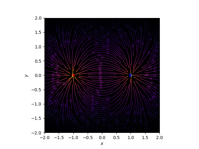
Figure 1: Illustration of Gauss's Law, which proposes that $div E = \frac{\rho}{\epsilon_{0}}$ |
HistoryIt is widely believed that Hamilton's study of quaternions is what prompted the development of vector calculus. Hamilton even used the dot and cross product of vectors to define the quaternion. Years later, passionate about providing a mathematical framework for Maxwell's electromagnetic field theory, Gibbs and Heaviside, independent of each other, further developed vector algebra that involved the dot and cross product of multivariable functions. In the year 1883, Heaviside, in a paper on electricity defined divergence as div R = $\nabla R$. It is said that he borrowed nabla, $\nabla$, from Gibbs' definition of the same. 16 |
Pause and Ponder
Hint (or rather the answer itself!): Green's Theorem
17 |
|
18 |
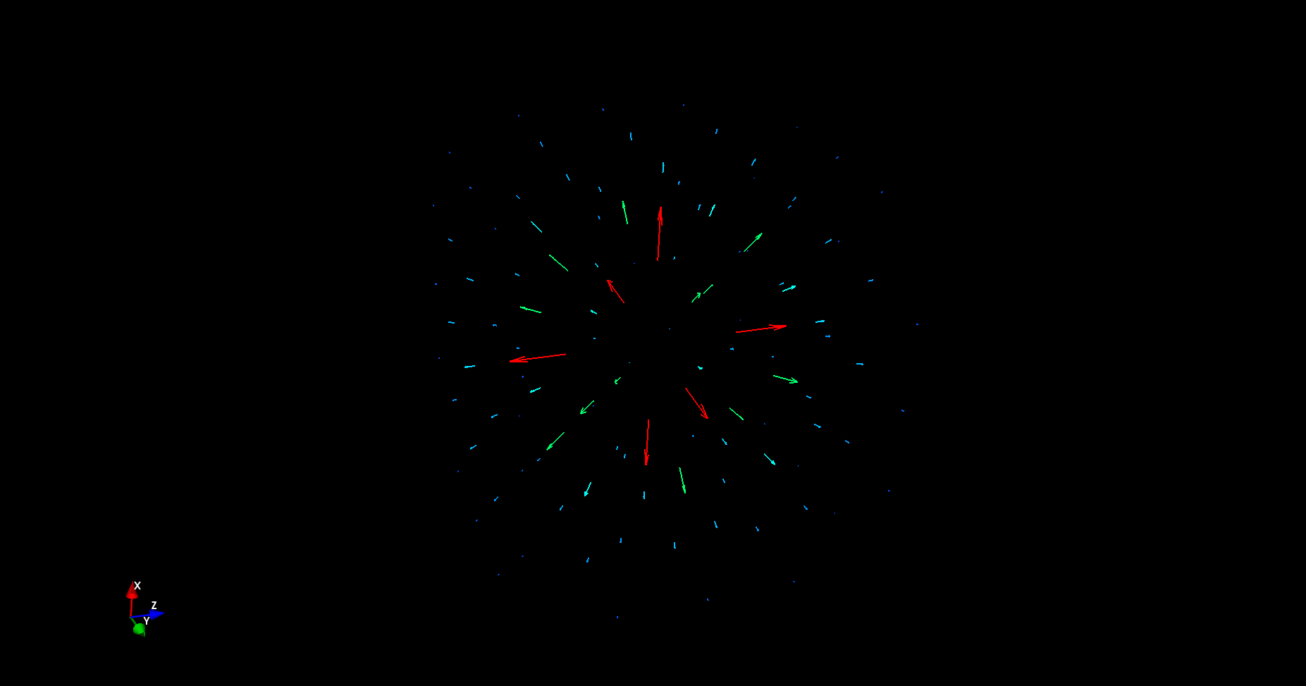
Figure 1: $\vec F = \frac{x,y,z}{\left(x^{2} + y^{2} + z^{2}\right) ^{3/2}}$ is a field that is seemingly outward flowing, but with zero divergence. |
19 |
|
20 |
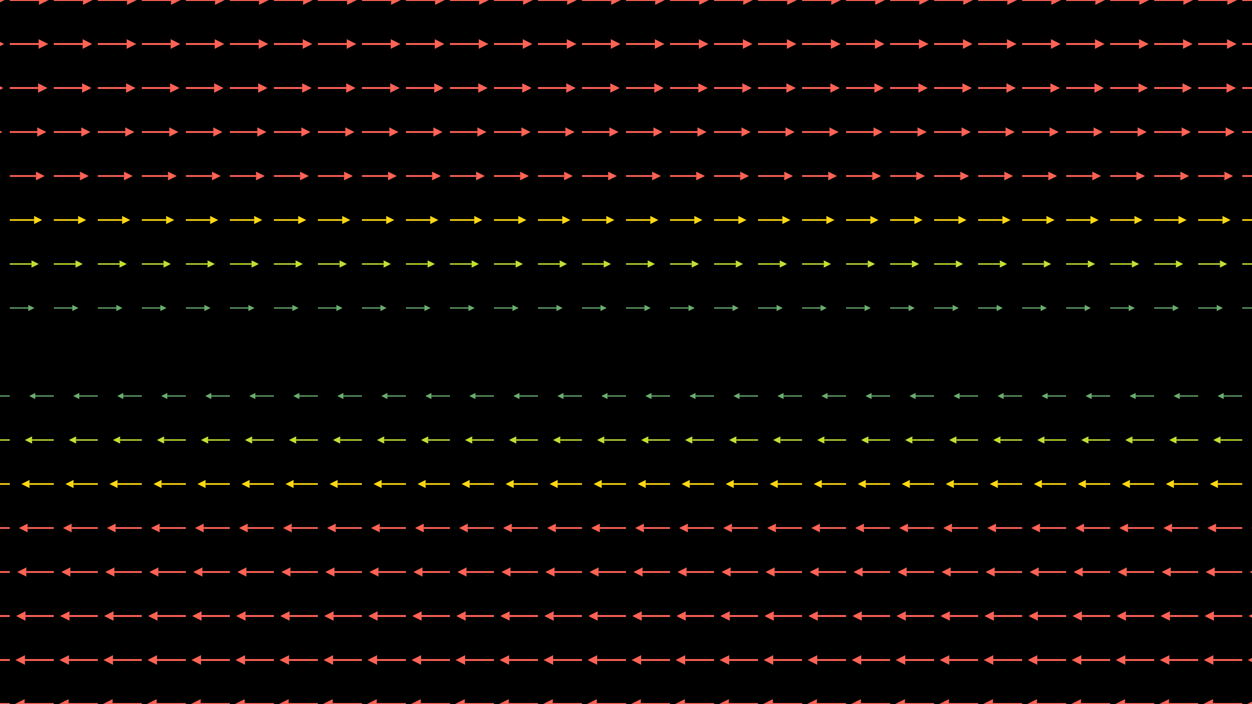
Figure 2: Does this vector field have any curl? (Note: The change in colour of the vector indicates its difference in speed. Red is the fastest, blue represents least velocity)) |
Further Reading
21 |
References
22 |
| Contributor: |
| Mentor & Editor: |
| Verified by: |
| Approved On: |
The following notes and their corrosponding animations were created by the above-mentioned contributor and are freely avilable under CC (by SA) licence. The source code for the said animations is avilable on GitHub and is licenced under the MIT licence.
