The Second Derivative Test |
|---|
DefinitionSuppose that $(a,b)$ is a critical point of function $z = f(x,y)$ so that $\frac{\partial f}{\partial x}(a,b) = \frac{\partial f}{\partial y}(a,b) =0$ and the second-order partial derivatives of $f$ are continuous in some region that contains (a,b). Let $H$ denote the "Hessian" matrix of second-order partial derivatives of $f$ : $$ H = \begin{equation*} \begin{bmatrix} \frac{\partial^2f}{\partial x^2} & \frac{\partial^2f}{\partial x\partial y}\\ \frac{\partial^2f}{\partial y\partial x} & \frac{\partial^2f}{\partial y^2} \end{bmatrix} \end{equation*} $$ Let $D_1 = \frac{\partial^2 f}{\partial x^2}$ or $\frac{\partial^2 f}{\partial y^2}$ and $D_2 = \text{det} (H) = \begin{equation} \frac{\partial^2f}{\partial x^2} \frac{\partial^2f}{\partial y^2} - \frac{\partial^2f}{\partial x\partial y}\frac{\partial^2f}{\partial y\partial x} \end{equation}$ $$\space$$ If $D_2(a,b)>0$ and $D_1(a,b)>0 $, then $f$ has a local minimum at $(a,b)$ $$\space$$ If $D_2(a,b)>0$ and $D_1(a,b)<0 $, then $f$ has a local maximum at $(a,b)$ $$\space$$ If $D_2 (a,b)<0$, then $f$ has a saddle point at $(a,b)$ $$\space$$ If $D_2 (a,b)=0$, then this result is inconclusive
-4 |
MotivationThe problem of determining the maximum or minimum of a function was one of the motivating factors in the development of Calculus in the seventeenth century. Since the first derivative test is only limited to finding the critical points of a function, in order to analyze the change in the value of the function (either increasing or decreasing) or to analyze the concavity of the function at the critical point, the second derivative test is employed. Considering the same output production function used in the lecture note of Critical Points, $Y= f(K, N)$ where $Y$ is the output of production dependent on capital input $K$ and labor input $N$. Suppose this function has a critical point $(K_0,N_0)$. Using the definition of the second derivative test, the point $(K_0, N_0)$ can be classified as either of the following: -4 |
|
-4 |
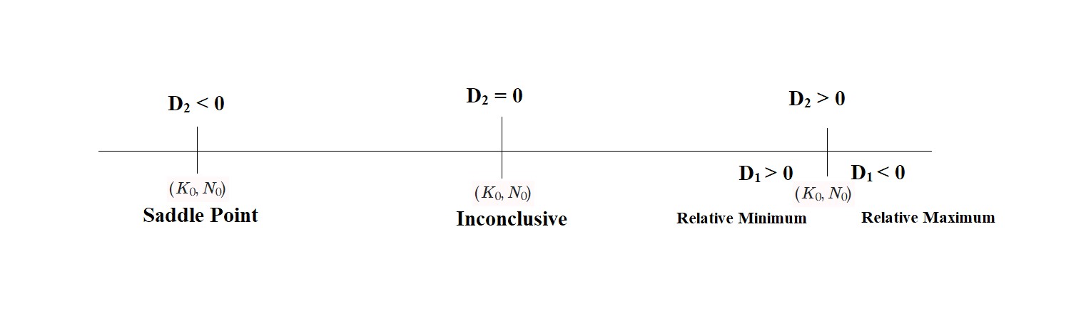
Figure 1: Second Derivative Test |
Bird's Eye ViewThe second derivative test uses the second-order partial derivatives ( $\frac{\partial^2 f}{\partial x^2}$,$\frac{\partial^2 f}{\partial y^2}$, $\frac{\partial^2 f}{\partial x \partial y}$, $\frac{\partial^2 f}{\partial y \partial x}$) to determine the concavity of the function at critical points. $\frac{\partial^2 f}{\partial x^2} = \frac{\partial}{ \partial x}(\frac{\partial f}{\partial x})$ measures the concavity of the function as the value of $x$ changes along $(\frac{\partial f}{\partial x})$ keeping $y$ constant. Similarly, $\frac{\partial^2 f}{\partial y^2} = \frac{\partial}{ \partial y}(\frac{\partial f}{\partial y})$ measures the concavity of the function as the value of $y$ changes along $(\frac{\partial f}{\partial y})$ keeping $x$ constant. $\frac{\partial^2 f}{\partial y \partial x} = \frac{\partial}{ \partial y}(\frac{\partial f}{\partial x})$ measures the “twist” of the graph as the value of $y$ changes along $\frac{\partial f}{\partial x}$ where $x$ is held constant. In the same way, $\frac{\partial^2 f}{\partial x \partial y} = \frac{\partial}{ \partial x}(\frac{\partial f}{\partial y})$ measures how the graph twists as the value of $x$ changes along $\frac{\partial f}{\partial y}$ where $y$ is held constant.
-4 |
|
-3 |
|
Video 1: Second order partial derivatives |
Context of DefinitionAs mentioned in the definition, $D_2 = \text{det} (H) = \begin{equation} \text{det}\begin{bmatrix} \frac{\partial^2f}{\partial x^2} & \frac{\partial^2f}{\partial x\partial y}\\ \frac{\partial^2f}{\partial y\partial x} & \frac{\partial^2f}{\partial y^2} \end{bmatrix} \end{equation}$ where $H$ denotes the Hessian Matrix. A Hessian Matrix is a square matrix of second-order partial derivatives of a function. If a multivariable function $f$ has $n$ number of second partial derivatives ($n$ measures of concavity), that is too many values to keep track of, so it would be nice to have some method to combine them. One of which is calculating the determinant of a Hessian matrix. A Hessian matrix can be classified into two types based on the signs of $\frac{\partial^2 f}{\partial x^2}$ and $\frac{\partial^2 f}{\partial y^2}$:
A Hessian matrix of a function \(f\) is nondegenerate when $\frac{\partial^2 f}{\partial x^2}\ne0$ and $\frac{\partial^2 f}{\partial y^2}\ne0$ This leads to three cases: case 1: Both $\frac{\partial^2 f}{\partial x^2}>0$ and $\frac{\partial^2 f}{\partial y^2}>0$ (relative minima) The value of the function increases on moving away from the critical point and the graph of the function is concave up at the critical point. $H_f = \begin{bmatrix} 2&0\\ 0&1 \end{bmatrix}$ case 2: Both $\frac{\partial^2 f}{\partial x^2}<0$ and $\frac{\partial^2 f}{\partial y^2}<0$ (relative maxima) The value of the function decreases on moving away from the critical point and the graph of the function is concave down at the critical point. $H_f = \begin{bmatrix} -2&0\\ 0&-1 \end{bmatrix}$ case 3: $\frac{\partial^2 f}{\partial x^2}$ and $\frac{\partial^2 f}{\partial y^2}$ have opposite signs(saddle point) The value of the function increases in one direction and decreases in the other and the graph of the function is concave up in one direction and concave down in the other. $H_f = \begin{bmatrix}-2&0\\ 0&1 \end{bmatrix}$
A Hessian matrix of a function $f$ is degenerate when $\frac{\partial^2 f}{\partial x^2}=0$ or $\frac{\partial^2 f}{\partial y^2}=0$ (inconclusive) $H_f = \begin{bmatrix}0&0\\ 0&-2 \end{bmatrix}$
-1 |
|
0 |
|
Video 2: Nondegenerate Hessian Matrix |
|
0 |
|
Video 3: Degenerate Hessian Matrix |
|
Now the question arises, "If the curvature and concavity of a function can be determined by the sign of $\frac{\partial^2 f}{\partial x^2}$ and $\frac{\partial^2 f}{\partial y^2}$, why to bother finding the determinant of Hessian Matrix?" Yes, it is possible to determine whether a critical point is relative maxima or relative minima or a saddle point from the signs of the second-order partial derivatives, but this is practical only for bi-variate functions. As the number of variables of a function increases, the number of higher-order partial derivatives also increases, so it becomes difficult to predict the concavity of the functionon the basis of the signs of all the higher-order partial derivatives. For a $n$-variate function, the generalized Hessian matrix would be $H_f=\begin{bmatrix} f_{11}&f_{12}&f_{13}&....&f_{1n}\\ f_{21}&f_{22}&f_{23}&....&f_{2n}\\.&.&.& &.\\.&.&.& &.\\f_{n1}&f_{n2}&f_{n3}&....&f_{nn}\\ \end{bmatrix}$ where $f_{11},f{12},....f_{nn}$ are the higher-order partial derivatives of $f$ Thus, computing determinant is a lot simpler in determining the concavity of the function. 0 |
CONTOUR DIAGRAMS:The contour diagram is one of the ways of representing a function of two variables. A contour is a projection of the surface of a function $z=f(x,y)$ on $x$ - $y$ plane where $z=k$ ( $z$ is constant) and only $x$ and $y$ vary. The surface which represents a function of two variables gives an idea of the function’s general behavior (whether it is increasing or decreasing as one of the variables increases). However, it is difficult to read numerical values off a surface and it can be hard to see all of the function’s behavior from a surface. Thus, the function of two variables is often represented by a contour diagram.
0 |
|
0 |
|
Video 4: Contour Diagram |
|
According to Figure 2, The leftmost Contour plot represents a saddle point at the critical point of the function $f(x,y)=x^2-2y^2-2x$. The Colormap on the right of the contour plot varies from positive to negative values corresponding to the color shade of the contour. The contour plot implies that the function at the saddle point is increasing in one direction and decreasing in the other. On moving either left or right (in the $x$-direction) of the critical point the value of $f$ increases and on moving either up or down (in the $y$-direction) from the critical point, the value of $f$ decreases. The middle Contour plot represents maxima at the critical point of the function $f(x,y)=-x^2-4y^2$. The Colormap on the right of the contour plot varies from 0 to negative values corresponding to the color shade of the contour. The contour plot implies that on moving away from the critical point in the $x$-$y$ plane, the value of $f$ decreases. The rightmost Contour plot represents minima at the critical point of the function $f(x,y)=2x^2+3y^2-2yx$. The Colormap on the right of the contour plot varies from positive values to 0, corresponding to the color shade of the contour. The contour plot implies that on moving away from the critical point in the $x$-$y$ plane, the value of $f$ increases. 0 |
|
0 |
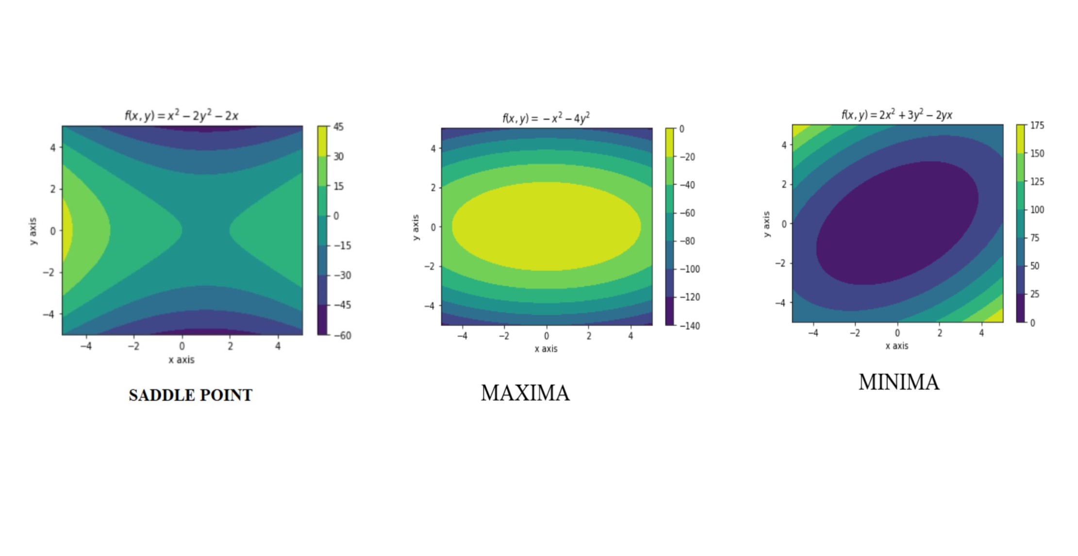
Figure 2 : Contour Diagrams [4] |
ApplicationsThe second derivative test determines the extrema and concavity of a function. This concept is used in Optimization problems (problems of finding maxima and minima of functions), which are among the most important problems in mathematics. They have extremely important applications in economics, engineering, and science. The second derivative test is useful in solving optimization problems like:
1 |
HistoryDuring the eighteenth and nineteenth centuries, Niklaus I Bernoulli, Clairaut, Euler, Fontaine, Lagrange, Gauss, Green, Cauchy, Ostrogradski, Jacobi, and others laid the foundations for the calculus of several variables. Most of this work was done in the context of mathematical physics. However, the traces of this subject goes back to the earliest work of both Newton and Leibniz. Newton expressed the curvature of $f(x,y)=0$ in terms of homogenized first and second-order partial derivatives of $f(x,y)$. He even worked out a notation for these partial derivatives. He described the method for finding the fluxional equation of $f(x,y)=0$, identical to the equation $\begin{equation} f_x \dot{x}+f_y \dot{y} =0\end{equation}$, where the dot notation denoted the derivative with respect to some parameter. Niklaus I defined both partial and complete differentials of variables depending upon a number of other variables. He proved the equality of mixed second-order differentials. In 1867, the Finnish mathematician Lorenz Lindelöf, presented a counterexample to show the proof that the mixed second derivatives were independent of their order. In 1873, H. A. Schwarz gave a proof of the equality of the mixed derivatives with fairly strong conditions on the partial derivatives. 1 |
Pause and Ponder
1 |
References$[1]$ https://www.iith.ac.in/~ashok/Maths_Lectures/TutorialB/Hessian_Examples.pdf $[2]$ https://math.okstate.edu/people/lebl/osu4013-s17/hessian.pdf $[3]$ https://ocw.mit.edu/courses/mathematics/18-02sc-multivariable-calculus-fall-2010 IMAGES: $[4]$ Contour plots in figure 2 are made using Matplotlib version 3.2.1 1 |
Further Reading
1 |
| Contributor: |
| Mentor & Editor: |
| Verified by: |
| Approved On: |
The following notes and their corrosponding animations were created by the above-mentioned contributor and are freely avilable under CC (by SA) licence. The source code for the said animations is avilable on GitHub and is licenced under the MIT licence.
